The computations of a neural network are organized in terms of a forward pass or a forward propagation step, in which we compute the output of the neural network, followed by a backward pass or back propagation step, which we use to compute gradients or compute derivatives.

The computation graph explains why it is organized this way.

In order to illustrate the computation graph, let's use a simpler example than logistic regression or a full blown neural network.

Let's say that we're trying to compute a function, J, which is a function of three variables a, b, and c and let's say that function is 3(a+bc) as shown below.

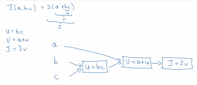
Computing this function actually has three distinct steps. The first is you need to compute what is bc and let's say we store that in the variable call u. So u=bc and then you my compute V=a *u. So let's say this is V. And then finally, your output J is 3V.

So this is your final function J that you're trying to compute.

We can take these three steps and draw them in a computation graph as given above.

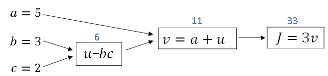
So as a concrete example, if a=5, b=3 and c=2 then u=bc would be six because a+u would be 5+6 is 11, J is three times that, so J=33.

So, the computation graph comes in handy when there is some distinguished or some special output variable, such as J in this case, that you want to optimize.

And in the case of a logistic regression, J is of course the cost function that we're trying to minimize. And what we're seeing in this little example is that, through a left-to-right pass, you can compute the value of J.

And in order to compute derivatives, there'll be a right-to-left pass like this, kind of going in the opposite direction as the blue arrows (shown below with red arrows).

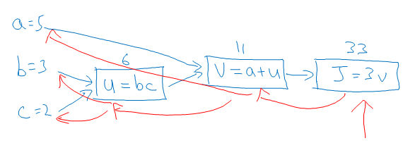
That would be most natural for computing the derivatives. So to recap, the computation graph organizes a computation with this blue arrow, left-to-right computation.

Let's say you want to compute the derivative of J with respect to v for the computation graph shown below.

In other words if we were to take the value of v and change it a little bit, how would the value of J change?

As J is defined as 3 times v (3*v). And, v = 11. So if we're to increase v by 11.001, then J, which is 3v, so currently 33, will get bumped up to 33.003.

So here, we've increased v by 0.001. And the net result of that is that J goes out 3 times as much. We conclude that the derivative of J with respect to v is equal to 3.

Because the increase in J is 3 times the increase in v. Here we have J = 3v, and so dJ/dv = 3.

In terminology of backpropagation, what we're seeing is that if you want to compute the derivative of this final output variable, which usually is a variable you care most about, with respect to v, then we've done one step of backpropagation.

So we call it one step backwards in this graph. Now let's look at another example. What is dJ/da? In other words, if we bump up the value of a, how does that affect the value of J?

Well, let's go through the example, where now a = 5. So let's bump it up to 5.001. The net impact of that is that v, which was a + u, so that was previously 11.

This would get increased to 11.001. And then we've already seen as above that J now gets bumped up to 33.003. So what we're seeing is that if you increase a by 0.001, J increases by 0.003. And by increase 'a', you have to take this value of 5 and just plug in a new value.

Then the change to 'a' will propagate to the right of the computation graph so that J ends up being 33.003. And so the increase to J is 3 times the increase to 'a'.

So that means this derivative is equal to 3. And one way to break this down is to say that if you change a, then that will change v.

And through changing v, that would change J. And so the net change to the value of J when you bump up the value, when you nudge the value of a up a little bit, is that,

First, by changing 'a', you end up increasing v. It is increased by an amount that's determined by dv/da. And then the change in v will cause the value of J to also increase. So in calculus, this is actually called the chain rule that if a affects v, affects J, then the amounts that J changes when you nudge 'a' is the product of how much v changes when you nudge a times how much J changes when you nudge v.

So in calculus, again, this is called the chain rule. And what we saw from this calculation is that if you increase a by 0.001, v changes by the same amount. So dv/da = 1.

So if you plug in what we have wrapped up previously, dv/dJ = 3 and dv/da = 1. So the product of these 3 times 1, that actually gives you the correct value that dJ/da = 3.

This little illustration shows hows by having computed dJ/dv, that is, derivative with respect to this variable, it can then help you to compute dJ/da. And that's another step of this backward calculation.

Now let's keep computing derivatives. Let's look at the value u. So what is dJ/du? Through a similar calculation as what we did before and then we start off with u = 6. If you bump up u to 6.001, then v, which is previously 11, goes up to 11.001. And so J goes from 33 to 33.003.

And so the increase in J is 3x, so this is equal. And the analysis for u is very similar to the analysis we did for 'a'. This is actually computed as dJ/dv times dv/du, where this we had already figured out was 3.

And this turns out to be equal to 1. So we've gone up one more step of backpropagation. We end up computing that dJ/du is also equal to 3.

So what is dJ/db? Imagine if you are allowed to change the value of b. And you want to tweak b a little bit in order to minimize or maximize the value of J. So what is the derivative or what's the slope of this function J when you change the value of b a little bit?

It turns out that using the chain rule for calculus, this can be written as the product of two things. This dJ/du times du/db.

The reasoning is if you change b a little bit, so b = 3 to, say, 3.001. The way that it will affect J is it will first affect u. So how much does it affect u?

Here u is defined as b times c. So this will go from 6, when b = 3, to now 6.002 because c = 2 in our example here. And so this tells us that du/db = 2. Because when you bump up b by 0.001, u increases twice as much. So du/db, this is equal to 2.

And now, we know that u has gone up twice as much as b has gone up. Well, what is dJ/du? This is equal to 3. And so by multiplying these two out, we find that dJ/db = 6. And again, here's the reasoning for the second part of the argument.

Which is we want to know when u goes up by 0.002, how does that affect J? The fact that dJ/du = 3, that tells us that when u goes up by 0.002, J goes up 3 times as much.

So J should go up by 0.006. So this comes from the fact that dJ/du = 3. And if you check the math in detail, you will find that if b becomes 3.001, then u becomes 6.002, v becomes 11.002.

So that's a + u, so that's 5 + u. And then J, which is equal to 3 times v, that ends up being equal to 33.006. And so that's how you get that dJ/db = 6. And to fill that in, this is if we go backwards, so this is db = 6.

Finally, if you also compute out dJ, this turns out to be dJ/du times du. And this turns out to be 9, this turns out to be 3 times 3. I won't go through that example in detail. So through this last step, it is possible to derive that dc is equal to.

So the key takeaway from this example, is that when computing derivatives the most efficient way to do so is through a right to left computation.

And in particular, we'll first compute the derivative with respect to v. And then that becomes useful for computing the derivative with respect to 'a' and the derivative with respect to u.

And then the derivative with respect to u in turn become useful for computing the derivative with respect to b and the derivative with respect to c.

So that was the computation graph and how does a forward or left to right calculation to compute the cost function such as J that you might want to optimize.

And a backwards or a right to left calculation to compute derivatives.