You can vectorize the implementation of logistic regression, so they can process an entire training set, that is implement a single elevation of grading descent with respect to an entire training set without using even a single explicit for loop.

Let's first examine the four propagation steps of logistic regression. So, if you have M training examples, then to make a prediction on the first example, you need to compute Z.

\( 𝑧^{(1)} = 𝑤^𝑇 𝑥^{(1)}+𝑏 \\ a^{(1)} = \sigma(𝑧^{(1)}) \\ 𝑧^{(2)} = 𝑤^𝑇 𝑥^{(2)}+𝑏 \\ a^{(2)} = \sigma(𝑧^{(2)}) \\ 𝑧^{(3)} = 𝑤^𝑇 𝑥^{(3)}+𝑏 \\ a^{(3)} = \sigma(𝑧^{(3)}) \\ \)

The above code tells how to compute Z and then the activation for three examples.

And you might need to do this M times, if you have M training examples.

So in order to carry out the four propagation step, that is to compute these predictions on our M training examples, there is a way to do so, without needing an explicit for loop.

First , we defined a matrix capital X to be our training inputs, stacked together in different columns like shown below.

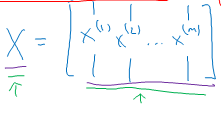
This is a (N_X by M) matrix.

Using this matrix we can compute \( Z = Z^{(1)} Z^{(2)} Z^{(3)} ... Z^{(n)}\) with one line of code. The matrix Z is a 1 by M matrix that's really a row vector.

Using matrix multiplication \( Z = W^TX + b \) can be computed to obtain Z in one step.

The python command is : z = np.dot(w.T, X) + B

Here W = (N_X by 1), X is (N_X by M) and b is (1 by M), multiplication and addition gives Z (1 by M).

Now there is a subtlety in Python , which is at here B is a real number or if you want to say you know 1x1 matrix, is just a normal real number.

But, when you add this vector to this real number, Python automatically takes this real number B and expands it out to this 1XM row vector.

This is called broadcasting in Python.

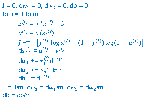
We can use vectorization to also perform the gradient computations for all M training samples. To derive a very efficient implementation of logistic regression.

For the gradient computation , the first step is to compute \( dz^{(1)} \) for the first example, which could be \( a^{(1)} - y^{(1)} \) and then \( dz^{(2)} = a^{(2)} - y^{(2)} \) and so on. And so on for all M training examples.

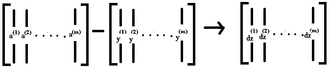
Lets define a new variable , dZ is going to be \( dz^{(1)}, dz^{(2)}, ... , dz^{(m)} \). Again, all the D lowercase z variables stacked horizontally. So, this would be 1 by m matrix or alternatively a 'm' dimensional row vector.

Previously , we'd already figured out how to compute A and Y as shown below and you can see for yourself that dz can be computed as just A minus Y because it's going to be equal to a1 - y1, a2 - y2, and so on.

So, with just one line of code , you can compute all of this at the same time. By a simple matrix multiplication as shown below.

Now after dz we compute dw₁, dw₂ and db as shown in the below figure.

To compute dw , we initialize dw to zero to a vector of zeroes. Then we still have to loop over examples where we have dw + = x₁ * dz₁, for the first training example and so on.

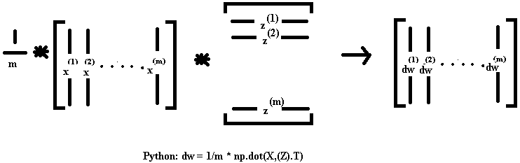
The above code line can vectorize the entire computation of dw in one line.

Similarly for the vectorize implementation of db was doing is basically summing up, all of these dzs and then dividing by m. This can be done using just one line in python as: db = 1/m * np.sum(dz)

And so the gradient descent update then would be you know W gets updated as w minus the learning rate times dw which was just computed above and B is update as B minus the learning rate times db.

Sometimes it's pretty close to notice that it is an assignment, but I guess I haven't been totally consistent with that notation. But with this, you have just implemented a single elevation of gradient descent for logistic regression.

Now, I know I said that we should get rid of explicit full loops whenever you can but if you want to implement multiple adjuration as a gradient descent then you still need a full loop over the number of iterations. So, if you want to have a thousand deliberations of gradient descent, you might still need a full loop over the iteration number.

There is an outermost full loop like that then I don't think there is any way to get rid of that full loop.

A technique in python which makes our code easy for implementation is called broadcasting