The second layer of the neural network has a matrix \( W^{[2]} \) with dimensions 1 * 4. The four columns are the weights multiplied with the vector of activations from hidden layer \( a^{[1]} \).

From the figure, we can see four incoming connections and hence one weight is assigned per connection.

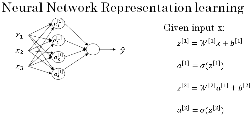
The operations performed for implementation of forward propagation are given below:

Using simple matrix operations we can implement a neural network.

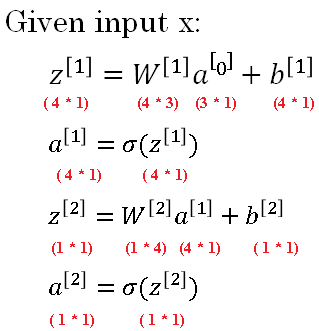
The dimensions of the matrix have to be aligned to avoid mismatch error.

In the last section, we saw how to compute the prediction on a neural network, given a single training example.

In this section, we see how to vectorize across multiple training examples. And the outcome will be quite similar to what we saw for logistic regression. Whereby stacking up different training examples in different columns of the matrix, you'd be able to take the equations you had from the previous section.

And with very little modification, change them to make the neural network compute the outputs on all the examples on pretty much all at the same time.

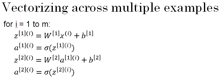
These were the four equations we have from the previous as shown below:

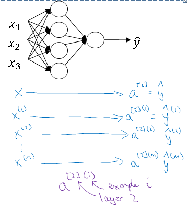
Now if you have "m" training examples, you need to repeat this process for say, the first training example. \( x^{(1)} \) to compute \( \hat{y}^{(1)} \) does a prediction on your first training example. Then \( x^{(2)} \) use that to generate prediction \( \hat{y}^{(1)} \). And so on down to \( x^{(m)} \) to generate a prediction \( \hat{y}^{(m)} \).

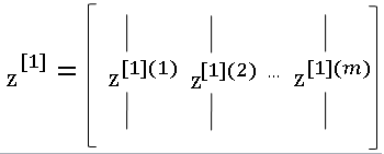
Since it is a two layered network \( \hat{y}^{(1)} \) is also known as \( a^{[2](1)} \).

Here, the superscript [2] means Layer-2 and (1) identifies the training example number (1). This process is also shown in below figure:

And so to suggest that if you have an unvectorized implementation and want to compute the predictions of all your training examples, you need to do the below code:

So as to get rid of this for-loop, we defined the matrix x to be equal to our training examples stacked up in these columns like so. So take the training examples and stack them in columns. So this becomes a \( n_x * m \) dimension matrix.

As we see below, the term n_x represents the number of features per example. 'm' refers to all the training examples in the data-set.

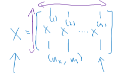
To implement the vectorised version of the code, we write the below lines. Here X is the input training examples stacked as columns as shown in above figure.

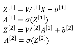
The matrix multiplication of \( W^{[1]}X + b^{[1]} \) gives the matrix Z. As shown below:

Appling the sigmoid operation element wise to \( Z^{[1]} \) shall give \( A^{[1]} \).