We will list the equations you need to implement in order to get back-propagation or to get gradient descent working, and then in next section give some more intuition about why these particular equations are the accurate equations for computing the gradients you need for your neural network.

So, your neural network, with a single hidden layer for now, will have parameters \( W^{[1]}, B^{[1]}, W^{[2]}, and B^{[2]} \).

For instance, if you have \( N_X \) or \( N^{[0]} \) input features, and \( N^{[1]} \) hidden units, and \( N^{[2]} \) output units in our examples.

Then the matrix \( W^{[1]} \) will be \( N^{[1]} * N^{[0]} \). \( B^{[1]} \) will be an \( N^{[1]} \) dimensional vector, so we can write that as \( N^{[1]} * 1 \) -dimensional matrix i.e. a column vector.

The dimensions of \( W^{[2]} \) will be \( N^{[2]} * N^{[1]} \) , and the dimension of \( B^{[2]} \) will be \( N^{[2]} * 1 \).

So far we've only seen examples where \( N^{[2]} \) is equal to one, where you have just one single hidden unit. Also have a cost function for a neural network. For now, I'm just going to assume that you're doing binary classification.

So, in that case, the cost of your parameters as follows is going to be \( \sum_{i = 1}^{m} L(a, y) \) i.e. one over M of the average of that loss function.

L here is the loss when your neural network predicts \( \hat{y} \). This is really \( A^{[2]} \) when the gradient label is equal to Y.

If you're doing binary classification, the loss function can be exactly what you use for logistic regression (cross-entropy loss).

To train the parameters of your algorithm, you need to perform gradient descent.

When training a neural network, it is important to initialize the parameters randomly rather than to all zeros.

The following steps are needed to implement gradient descent in neural networks:

The below equations implement gradient descent for a neural network:
\( 𝑑𝑧^{[2]}=𝑎^{[2]}−𝑦 \\ 𝑑𝑊^{[2]} =𝑑𝑧^{[2]} 𝑎^{[1]^𝑇}\\ 𝑑𝑏^{[2]}=𝑑𝑧^{[2]} \\ 𝑑𝑧^{[1]}=𝑊^{[2]^𝑇} 𝑑𝑧^{[2]}∗𝑔^{[1]}′(z^{[1]} ) \\ 𝑑𝑧^{[1]}=𝑊^{[2]^𝑇} 𝑑𝑧^{[2]}∗𝑔^{[1]}′(z^{[1]} ) \\ 𝑑𝑧^{[1]}=𝑊^{[2]^𝑇} 𝑑𝑧^{[2]}∗𝑔^{[1]}′(z^{[1]} ) \\ 𝑊^{[2]} = 𝑊^{[2]} - \alpha * 𝑑𝑊^{[2]} \\ B^{[2]} = B^{[2]} - \alpha * 𝑑B^{[2]} \\ 𝑊^{[1]} = 𝑊^{[1]} - \alpha * 𝑑𝑊^{[1]} \\ B^{[1]} = B^{[1]} - \alpha * 𝑑B^{[1]} \\ \)

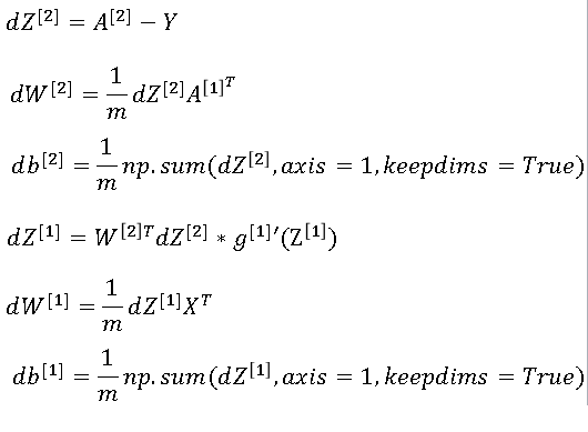
The above code can be implemented in python to run gradient descent for your neural network.

When you train your neural network, it's important to initialize the weights randomly.

For logistic regression, it was okay to initialize the weights to zero. But for a neural network of initialize the weights to parameters to all zero and then applied gradient descent, it won't work.

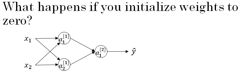
So you have here two input features, so \( n^{[0]} = 2 \), and two hidden units, so \( n^{[1]} = 2 \). And so the matrix associated with the hidden layer, \( W^{[1]} = 2 * 2 \), is going to be two-by-two.

Let's say that you initialize it to all 0s. And let's say \( B^{[1]} \) is also equal to 0.

It turns out initializing the bias terms b to 0 is actually okay, but initializing w to all 0s is a problem.

The solution to this is to initialize your parameters randomly.

You can set \( W^{[1]} = 2 * 2 \) (np.random.randn). This generates a gaussian random variable (2,2). And then usually, you multiply this by very small number, such as 0.01.

So you initialize it to very small random values. And then b, it turns out that b does not have the symmetry problem

So it's okay to initialize b to just zeros. Because so long as w is initialized randomly, you start off with the different hidden units computing different things.

And so you no longer have this symmetry breaking problem. And then similarly, for w2, you're going to initialize that randomly. And b2, you can initialize that to 0.

The constant for multiplication is 0.01 as we usually prefer to initialize the weights to very small random values.

Because if you are using a tanh or sigmoid activation function then If the weights are too large, then when you compute the activation values it will be either very large or very small.

And so in that case, you're more likely to end up at these end parts of the tanh function or the sigmoid function, where the slope or the gradient is very small. Meaning that gradient descent will be very slow.

So learning would be very slow.

If you don't have any sigmoid or tanh activation functions throughout your neural network, this is less of an issue. But if you're doing binary classification, and your output unit is a sigmoid function, then you just don't want the initial parameters to be too large.

So that's why multiplying by 0.01 would be something reasonable to try, or any other small number.