When implementing a deep neural network, one of the debugging tools often used to check the correctness of the code is work through the dimensions and matrix involved.

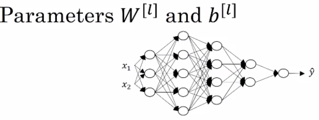
In above figure, Capital L is equal to 5, i.e. not counting the input layer, there are five layers here, so four hidden layers and one output layer.

And so if you implement forward propagation, the steps will be: \( Z^{[1]} = W^{[1]}*A^{[0]} + B^{[1]} \\ A^{[1]} = g(Z^{[1]}) \\ Z^{[2]} = W^{[2]}*A^{[1]} + B^{[2]} \\ A^{[2]} = g(Z^{[2]}) \\ Z^{[3]} = W^{[3]}*A^{[2]} + B^{[3]} \\ A^{[3]} = g(Z^{[3]}) \\ Z^{[4]} = W^{[4]}*A^{[3]} + B^{[4]} \\ A^{[4]} = g(Z^{[4]}) Z^{[5]} = W^{[5]}*A^{[4]} + B^{[5]} \\ \hat{Y} = A^{[5]} = g(Z^{[5]}) \\ \)

Now this first hidden layer has three hidden units. So using the notation we had from the previously, we have that \( n^{[1]} \), which is the number of hidden units in layer 1, is equal to 3.

And here we would have the \( n^{[2]} \) is equal to 5, \( n^{[3]} \) is equal to 4, \( n^{[4]} \) is equal to 2, and \( n^{[5]} \) is equal to 1.

And finally, for the input layer, we also have \( n^{[0]} \) = n_x = 2.

So now, let's think about the dimensions of z, w, and x. z is the vector of activations for this first hidden layer, so z is going to be 3 by 1, it's going to be a 3-dimensional vector.

So I'm going to write it a \( n^{[1]} \) by 1-dimensional vector, \( n^{[1]} \) by 1-dimensional matrix, all right, so 3 by 1 in this case.

Now about the input features x, we have two input features.

So x is in this example 2 by 1, but more generally, it would be \( n^{[0]} \) by 1.

So what we need is for the matrix \( w^{[1]} \) to be something that when we multiply an \( n^{[0]} \) by 1 vector to it, we get an \( n^{[1]} \) by 1 vector

So you have a three dimensional vector equals something times a two dimensional vector.

And so by the rules of matrix multiplication, this has got be a 3 by 2 matrix because a 3 by 2 matrix times a 2 by 1 matrix, or times the 2 by 1 vector, that gives you a 3 by 1 vector.

And more generally, this is going to be an \( n^{[1]} \) by \( n^{[0]} \) dimensional matrix.

So what we figured out here is that the dimensions of \( w^{[1]} \) has to be \( n^{[1]} \) by \( n^{[0]} \).

And more generally, the dimensions of \( w^{[L]} \) must be \( n^{[L]} \) by \( n^{[L]} \) minus 1. So for example, the dimensions of \( w^{[2]} \) , for this, it would have to be 5 by 3, or it would be \( n^{[2]} \) by \( n^{[1]} \). Because we're going to compute \( z^{[2]} \) as \( w^{[2]} \) times \( a^{[1]} \) (let's ignore the bias for now).

So the general formula to check is that when you're implementing the matrix for layer L, that the dimension of that matrix be \( n^{[L]} \) by \( n^{[L-1]} \).

Let's think about the dimension of this vector b. The general rule is that \( b^{[L]} \) should be \( n^{[L]} \) by 1 dimensional.

So hopefully these two equations help you to double check that the dimensions of your matrices w, as well as your vectors p, are the correct dimensions.

And of course, if you're implementing back propagation, then the dimensions of dw should be the same as the dimension of w.

So dw should be the same dimension as w, and db should be the same dimension as b.

Now the other key set of quantities whose dimensions to check are these z, x, as well as \( a^{[L]} \) because \( z^{[L]} \) is equal to \( g(a^{[L]} \), applied element wise, then z and a should have the same dimension in these types of networks.