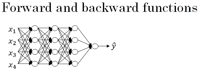
Building blocks of deep neural networks
Below is a network of a few layers. Let's pick one layer.
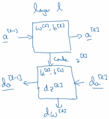
And look into the computations focusing on just that layer for now. So for layer L, you have some parameters \( w^{[l]} \) and \( b^{[l]} \) and for the forward prop, you will input the activations \( a^{[l-1]} \) from your previous layer and output \( a^{[l]} \).
We compute \( z^{[l]} = w^{[l]} * a^{[l-1]} + b^{[l]} \) . And then \( a^{[l]} = g(z^{[l]}) \) .
So, you go from the input \( a^{[l-1]} \) to the output \( a^{[l]} \).
For later use it'll be useful to also cache the value \( z^{[l]} \) for the back propagation step.
And then for the backward step or for the back propagation step, again, focusing on computation for this layer l, you're going to implement a function that inputs \( da^{[l]} \) and outputs \( da^{[l-1]} \)
So just to summarize, in layer l, you're going to have the forward step or the forward prop of the forward function. Input \( a^{[l-1]} \) and output \( a^{[l]} \) and in order to make this computation you need to use \( w^{[l]} \) and \( b^{[l]} \).
Then the backward function, using the back prop step, will be another function that now inputs \( da^{[l]} \) and outputs \( da^{[l-1]} \).
If you can implement these two functions then the basic computation of the neural network will be as follows.
You're going to take the input features \( a^{[0]} \), feed that in, and that would compute the activations of the first layer \( a^{[1]} \) and to do that we need a \( w^{[1]} \) and \( b^{[1]} \) and then will also cache \( z^{[1]} \).
Continuing till the last layer, you end up outputting \( a^{[l]} \) which is equal to \( \hat{y} \). During this process, we cached all of these values z.
Now, for the back propagation step, we are going backwards and computing gradients like so.
We feed in \( da^{[l]} \) and then this box will give us \( da^{[l-1]} \) and so on until we get \( da^{[1]} \).
Along the way, backward prop also ends up outputting \( dw^{[l]}, db^{[l]}, dz^{[l]} \).
So one iteration of training through a neural network involves many computations as shown below in the figure. We store in the cache the values \( w^{[l]}, b^{[l]}, z^{[l]} \). As they are useful in the backward propagation step.
-
In the next section, we'll talk about how you can actually implement these building blocks.