This is a learning algorithm that you use when the output labels Y in a supervised learning problem are all either zero or one i.e. binary classification problems.

Given an input feature vector X maybe corresponding to an image that you want to recognize as either a cat picture or not a cat picture, you want an algorithm that can output a prediction, \( \hat{y} \), which is known as estimate of Y.

More formally, you want \( \hat{y} \) to be the probability of the chance that, Y is equal to one given the input features X. So in other words, if X is a picture you want \( \hat{y} \) to tell you, what is the chance that this is a cat picture?

Given x, \( \hat{y} = P( y = 1 | x), where 0 \leq \hat{y} \leq 1 \)

The parameters used in Logistic regression are:

The input features vector: \( x \in R^{n_x} \) where \( n_x \) is the number of features.

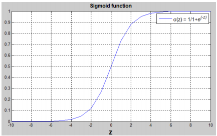
\( (w^Tx + b) \) is a linear function (ax + b), but since we are looking for a probability constraint between [0,1], the sigmoid function is used. The function is bounded between [0,1] as shown in the graph above.

Some observations from the graph:

So from previous data X is an X dimensional vector, given that the parameters of logistic regression will be W which is also an X dimensional vector, together with b which is just a real number.

So given an input X and the parameters W and b, how do we generate the output \( \hat{y} \)? Well, one thing you could try, that doesn't work, would be to have \( \hat{y} \) be w transpose X plus B \( (w^Tx + b) \), is a linear function of the input X.

But this isn't a very good algorithm for binary classification because you want \( \hat{y} \) to be the chance that Y is equal to one. So \( \hat{y} \) should really be between zero and one, and it's difficult to enforce that because W transpose X plus B can be much bigger then one or it can even be negative, which doesn't make sense for probability, that you want it to be between zero and one.

So in logistic regression our output is instead going to be \( \hat{y} \) equals the sigmoid function applied to this quantity. This is what the sigmoid function looks like (figure below).

It goes smoothly from zero up to one. When you implement logistic regression, your job is to try to learn parameters W and B so that \( \hat{y} \) becomes a good estimate of the chance of Y being equal to one.

To train the parameters 𝑤 and 𝑏, we need to define a cost function.

Recap: \( \hat{y}^{(i)} = \sigma(w^Tx^{(i)} + b) \), where \( \sigma(z^{(i)}) = \frac{1}{1 + e^{-z^{(i)}}} \)

\( x^{(i)} \) the i-th training example

Given \( {(x^{(1)}, y^{(1)}), (x^{(2)}, y^{(2)}), ... , (x^{(m)}, y^{(m)})} \), we want \( \hat{y^{(i)}} \sim y^{(i)} \)

Loss (error) function: The loss function measures the discrepancy between the prediction \( \hat{y}^{(i)}\) and the desired output (y^{(i)}). In other words, the loss function computes the error for a single training example.

\( L(\hat{y}^{(i)}, y^{(i)}) = \frac{1}{2} (\hat{y}^{(i)} - y^{(i)})^2 \)

\( L(\hat{y}^{(i)}, y^{(i)}) = -(y^{(i)} log(\hat{y}^{(i)}))+(1 - y^{(i)})log(1 - \hat{y}^{(i)}) \)

If \( y^{(i)} = 1; L(\hat{y}^{(i)}, y^{(i)}) = -log(\hat{y}^{(i)}) \) where \( log(\hat{y}^{(i)}) \) and \( \hat{y}^{(i)} \) should be close to 1

If \( y^{(i)} = 0; L(\hat{y}^{(i)}, y^{(i)}) = -log(1 - \hat{y}^{(i)}) \) where \( log(1 - \hat{y}^{(i)}) \) and \( \hat{y}^{(i)} \) should be close to 0

Cost function

The cost function is the average of the loss function of the entire training set. We are going to find the parameters w,b that minimize the overall cost function.

\( J(w,b) = − \frac{1}{m} \sum_{i = 1}^{m} L(\hat{y}^{(i)}, y^{(i)}) = − \frac{1}{m} \sum_{i = 1}^{m} [y^{(i)}log(\hat{y}^{(i)})−(1−y^{(i)})log(1−\hat{y}^{(i)}) ] \)