When you implement back propagation you'll find that there's a test called gradient checking that can really help you make sure that your implementation of back prop is correct.

Because sometimes you write all these equations and you're just not 100% sure if you've got all the details right and internal back propagation.

So in order to build up to gradient and checking, let's first talk about how to numerically approximate computations of gradients and in the next section, we'll talk about how you can implement gradient checking to make sure the implementation of backdrop is correct.

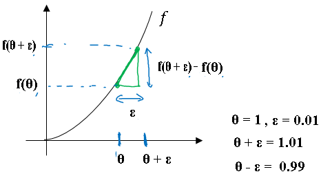
So lets take the function f and replot it below and remember this is \( f(\theta) = \theta^3 \), and let's again start off to some value of theta.

Let's say theta equals 1. Now instead of just nudging \( \theta \) (theta) to the right to get \( \theta + \epsilon \) (theta + epsilon), we're going to nudge it to the right and nudge it to the left to get \( \theta - \epsilon \) (theta + epsilon), as was \( \theta + \epsilon \) (theta + epsilon).

Plotting the values we get below figure:

It turns out that rather than taking this little triangle and computing the height over the width, you can get a much better estimate of the gradient if you take the below estimation.

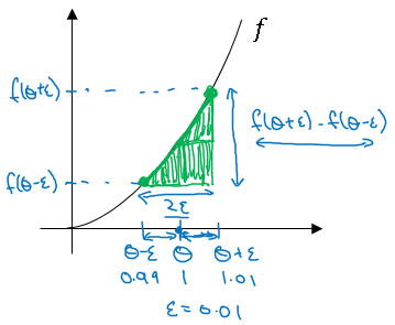
So for technical reasons which we won't go into, the height over width of this bigger green triangle gives you a much better approximation to the derivative at theta.

So rather than a one sided difference, you're taking a two sided difference.

So let's work out the math. For the bigger triangle shown, the height divided by the width is given by below formula:

\( \frac{f(\theta + \epsilon) + f(\theta - \epsilon)}{2 * \epsilon} \)

And this should hopefully be close to \( g(\theta) \). So plug in the values, remember \( f(\theta) = \theta^3 \).

\( \frac{f(\theta + \epsilon) + f(\theta - \epsilon)}{2 * \epsilon} \sim g(\theta) \\ \frac{(1.01)^3 - (0.99)^3}{2 * (0.01)}\\ = 3.0001 \\ g(\theta) = 3(\theta)^2 = 3\\ 3.0001 \sim 3 \)

The approximate error is 0.0001

So you've seen how by taking a two sided difference, you can numerically verify whether or not a function g, g of theta that someone else gives you is a correct implementation of the derivative of a function f.

Let's now see how we can use this to verify whether or not your back propagation implementation is correct or if there might be a bug in there that you need to go and ease out

Gradient checking is a technique that's helped save tons of time, and helped find bugs in implementations of back propagation many times.

Let's see how you could use it too to debug, or to verify that your implementation and back process correct.

So your new network will have some sort of parameters, \( W^{[1]}, W^{[2]},, ... , W^{[L]} \) AND \( b^{[1]}, b^{[2]},, ... , b^{[L]} \).

So to implement gradient checking, the first thing you should do is take all your parameters and reshape them into a giant vector data \( \theta \) (theta).

You gotta take all of these \( W^{[1]}, W^{[2]},, ... , W^{[L]} \) and \( b^{[1]}, b^{[2]},, ... , b^{[L]} \) and reshape them into vectors, and then concatenate all of these things, so that you have a giant vector theta (\theta).

So we say that the cost function J being a function of the Ws and Bs (\( W^{[1]}, W^{[2]},, ... , W^{[L]} \) AND \( b^{[1]}, b^{[2]},, ... , b^{[L]} \)), You would now have the cost function J being just a function of theta (\theta). Next, with W and B ordered the same way, you can also take dW[1], db[1] and so on, and initiate them into big, giant vector d-theta of the same dimension as theta.

So same as before, we shape dW[1] into the matrix, db[1] is already a vector. We shape dW[L], all of the dW's which are matrices.

Remember, dW1 has the same dimension as W1. db1 has the same dimension as b1. So the same sort of reshaping and concatenation operation, you can then reshape all of these derivatives into a giant vector d-theta.

Which has the same dimension as theta.

So here's how you implement gradient checking, and often abbreviate gradient checking to gradcheck.

So to implement grad check, what you're going to do is implements a loop so that for each component of theta, let's compute \( \frac{\partial J(\theta^+)}{\partial \theta} \) and two sided difference \( \frac{\partial J(\theta^-)}{\partial \theta} \).

\( \frac{\partial J}{\partial \theta} = \lim_{\varepsilon \to 0} \frac{J(\theta + \varepsilon) - J(\theta - \varepsilon)}{2 \varepsilon} \tag{1} \)

First compute "gradapprox" using the formula above (1) and a small value of \( \varepsilon \). Here are the Steps to follow:

1. \( \theta^{+} = \theta + \varepsilon \)
2. \( \theta^{-} = \theta - \varepsilon \)
3. \( J^{+} = J(\theta^{+}) \)
4. \( J^{-} = J(\theta^{-}) \)
5. \( gradapprox = \frac{J^{+} - J^{-}}{2 \varepsilon} \)

Then compute the gradient using backward propagation, and store the result in a variable "grad"

Finally, compute the relative difference between "gradapprox" and the "grad" using the following formula:

\( difference = \frac {\mid\mid grad - gradapprox \mid\mid_2}{\mid\mid grad \mid\mid_2 + \mid\mid gradapprox \mid\mid_2} \tag{2} \)

If this difference is small (say less than \( 10^{-7} \), you can be quite confident that you have computed your gradient correctly. Otherwise, there may be a mistake in the gradient computation.

Don’t use Gradient checking in training – only to debug

If algorithm fails grad check, look at components to try to identify bug.

Gradient checking Doesn’t work with dropout

Run at random initialization; perhaps again after some training.