Need for Optimization Techniques
In this section, you learn about optimization algorithms that will enable you to train your neural network much faster.
As we said before that applying machine learning is a highly empirical process, is highly iterative process.
In which you just had to train a lot of models to find one that works really well.
So, it really helps to really train models quickly.
One thing that makes it more difficult is that Deep Learning does not work best in a regime of big data.
We are able to train neural networks on a huge data set and training on a large data set is slow.
So, what you find is that having fast optimization algorithms, having good optimization algorithms can really speed up the efficiency of your team.
Mini-batch gradient descent
You've learned previously that vectorization allows you to efficiently compute on all m examples, that allows you to process your whole training set without an explicit for loops.
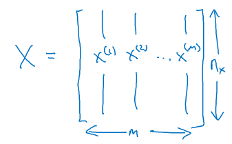
That's why we would take our training examples and stack them into these huge matrix X such that the columns of X are \( X^{[1]}, X^{[2]}, X^{[3]}, ... , X^{[M]} \) training samples.
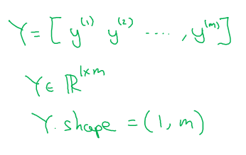
And similarly for Y this is \( Y^{[1]}, .... , Y^{[M]} \).
So, the dimension of X was an nx by M and Y was 1 by M. Where nx are the number of features of the training example. The two matrices can be shown with the below diagram.
Vectorization allows you to process all M examples relatively quickly but if M is very large then it can still be slow. For example what if M was 5 million or 50 million or even bigger.
With the implementation of gradient descent on your whole training set, what you have to do is, you have to process your entire training set before you take one little step of gradient descent.
And then you have to process your entire training sets of five million training samples again before you take another little step of gradient descent.
So, it turns out that you can get a faster algorithm if you let gradient descent start to make some progress even before you finish processing your entire, your giant training sets of 5 million examples.
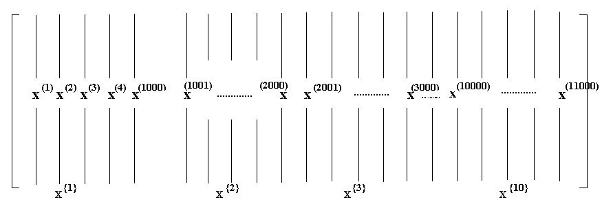
Mini-batch gradient descent allows you to do this. Let's say that you split up your training set into smaller, little baby training sets and these baby training sets are called mini-batches.
And let's say each of your baby training sets have just 1,000 examples each.
So, you take \( X^{[1]} ,....., X^{[1,000]} \) and you call that your first little baby training set, also call the mini-batch.
And then you take the next 1,000 examples. \( X^{[1001]} ,....., X^{[2,000]} \) as the next mini-batch and so on.
We are going to introduce a new notation for these mini-batches to call this \( X^{{1}} \) and I am going to call the second mini-batch \( X^{{2}} \).
Now, if you have 5 million training samples total and each of these little mini batches has a thousand examples, that means you have \( X^{{1}}, X^{{2}}, ... , X^{{5000}} \).
Then similarly you do the same thing for Y. You would also split up your training data for Y accordingly. So, \( Y^{{1}}, Y^{{2}}, ... , Y^{{5000}} \)
Now, mini batch number T is going to be comprised of \( X^{{T}}, Y^{{T}} \).
To explain the name of this algorithm, batch gradient descent, refers to the gradient descent algorithm we have been discussing about previously.
Where you process your entire training set all at the same time. And the name comes from viewing that as processing your entire batch of training samples all at the same time.
Mini-batch gradient descent in contrast, refers to algorithm in which you process is single mini batch \( X^{{T}}, Y^{{T}} \) at the same time rather than processing your entire training set \( X, Y \) the same time.
To run mini-batch gradient descent on your training sets you run for T equals 1 to 5,000 because we had 5,000 mini batches as high as 1,000 each.
    repeat
    {
        for t = 1, ..........., 5000
              {

              Forward propagation on X{t}
                      Z[1] = W[1]X{t} + b[1]
                      A[1] = g[1](Z[1])
                      .
                      .
                      .
                      .
                     A[L] = g[L](Z[L])
             Compute cost on X{t} as J{t}
             Backpropagation to compute gradients
             Update W and b
             } // after completion of loop 1 pass over training set over i.e. 1 epoch
    } // for multiple iterations over training set
What are you going to do inside the for loop is basically implement one step of gradient descent using \( X^{{T}}, Y^{{T}} \).
It is as if you had a training set of size 1,000 examples.
Let us write this out first, you implemented forward prop on the inputs \( X^{{T}} \) instead of X which is the entire training data-set.
It's just that this vectorized implementation processes 1,000 examples at a time rather than 5 million examples.
Next you compute the cost function J for the first mini batch \( X^{{T}}, Y^{{T}} \).
You notice that everything we are doing is exactly the same as when we were previously implementing gradient descent except that instead of doing it on X and Y, you're not doing it on \( X^{{T}}, Y^{{T}} \).
Next, you implement backward prop to compute gradients with respect to \( J^{{T}} \), you are still using only \( X^{{T}}, Y^{{T}} \) and then you update the weights W and similarly for B.
This is one pass through your training set using mini-batch gradient descent.
The code we have written down here is also called doing one epoch of training and epoch is a word that means a single pass through the training set.
Whereas with batch gradient descent, a single pass through the training allows you to take only one gradient descent step.
With mini-batch gradient descent, a single pass through the training set, that is one epoch, allows you to take 5,000 gradient descent steps.
Now of course you want to take multiple passes through the training set which you usually want to, you might want another for loop outside.
So you keep taking passes through the training set until hopefully you converge with approximately converge.
When you have a large training set, mini-batch gradient descent runs much faster than batch gradient descent and that's pretty much what everyone in Deep Learning will use when you're training on a large data set.
In the next section, let's delve deeper into mini-batch gradient descent so you can get a better understanding of what it is doing and why it works so well.