We want to show you a few optimization algorithms. They are faster than gradient descent.

In order to understand those algorithms, you need to be able they use something called exponentially weighted averages. Also called exponentially weighted moving averages in statistics.

Let's first discuss that, and then we'll use this to build up to more sophisticated optimization algorithms.

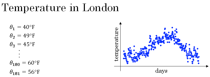
For this example we got the daily temperature from London from last year. So, on January 1, temperature was 40 degrees Fahrenheit. And on January 2, it was nine degrees Celsius and so on. And then about halfway through the year, sometime day number 180 will be sometime in late May. It was 60 degrees Fahrenheit.

So, it start to get warmer, towards summer and it was colder in January.

So, you plot the data you end up with this.

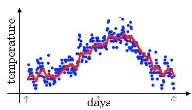
So, this data looks a little bit noisy and if you want to compute the trends, the local average or a moving average of the temperature, here's what you can do.

Let's initialize V₀ = 0. And then, on every day, we're going to average it with a weight of 0.9 times whatever appears as value, plus 0.1 times that day temperature. \( V_1 = 0.9V_0 + 0.1\theta_1 \)

So, \( \theta_1 \) (theta one) would be the temperature from the first day. And on the second day, we're again going to take a weighted average. 0.9 times the previous value plus 0.1 times today's temperature and so on.

And the more general formula is V on a given day is 0.9 times V from the previous day, plus 0.1 times the temperature of that day.

The formulae are as given below: \( V_0 = 0 \\ V_1 = 0.9V_0 + 0.1\theta_1 \\ V_2 = 0.9V_1 + 0.1\theta_2 \\ V_3 = 0.9V_2 + 0.1\theta_3 \\ . \\ . \\ . \\ . \\ V_t = 0.9V_{t-1} + 0.1\theta_t \)

So, if you compute this and plot it in red, this is what you get.

You get a moving average of what's called an exponentially weighted average of the daily temperature.

So, let's look at the equation we had from the previous section, it was \( V_t = 0.9V_{t-1} + 0.1\theta_t \).

\( V_0 = 0 \\ V_1 = 0.9V_0 + 0.1\theta_1 \\ V_2 = 0.9V_1 + 0.1\theta_2 \\ V_3 = 0.9V_2 + 0.1\theta_3 \\ . \\ . \\ . \\ . \\ V_t = 0.9V_{t-1} + 0.1\theta_t \)

We'll now turn that to 0.9 to beta, beta and 0.1 into one minus beta so, we get new equation as

\( V_t = \beta V_{t-1} + (1 - \beta) \theta_t \)

It turns out that when you compute this you can think of \(V_T\) as approximately averaging ove \( \frac{1}{1 - \beta} \) day's temperature.

So, for example when \( \beta \) goes 0.9 you could think of this as averaging over the last 10 days temperature \( \frac{1}{1 - \beta} = \frac{1}{1 - 0.9} = 10 \).

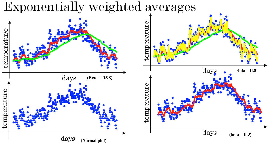
Now, let's try something else. Let's set beta to be very close to one, let's say it's 0.98. Then, if you look at \( \frac{1}{1 - \beta} = \frac{1}{1 - 0.98} = 50 \), this is equal to 50. So, this is, you know, think of this as averaging over roughly, the last 50 days temperature.

And if you plot that you get the green line. So, notice a couple of things with this very high value of beta. The plot you get is much smoother because you're now averaging over more days of temperature. So, the curve is just, you know, less wavy is now smoother, but on the flip side the curve has now shifted further to the right because you're now averaging over a much larger window of temperatures.

And by averaging over a larger window, this formula, this exponentially weighted average formula. It adapts more slowly, when the temperature changes.

So, there's just a bit more latency. And the reason for that is when Beta 0.98 then it's giving a lot of weight to the previous value and a much smaller weight just 0.02, to whatever you're seeing right now.

So, when the temperature changes, when temperature goes up or down, there's exponentially weighted average. Just adapts more slowly when beta is so large.

Now, let's try another value. If you set beta to another extreme, let's say it is 0.5, then this by the formula we have on the right.

This is something like averaging over just two days temperature, and you plot that you get this yellow line.

And by averaging only over two days temperature, you have a much, as if you're averaging over much shorter window. So, you're much more noisy, much more susceptible to outliers.

But this adapts much more quickly to what the temperature changes.

So, this formula is called an exponentially weighted moving average in the statistics literature.

We're going to call it exponentially weighted average for short and by varying this parameter or later we'll see such a hyper parameter if you're learning algorithm you can get slightly different effects and there will usually be some value in between that works best.

That gives you the red curve which you know maybe looks like a better average of the temperature than either the green or the yellow curve.

You now know the basics of how to compute exponentially weighted averages.

In the next section, let's get a bit more intuition about what it's doing.