You've learned how to implement exponentially weighted averages. There's one technical detail called bias correction that can make you computation of these averages more accurately.

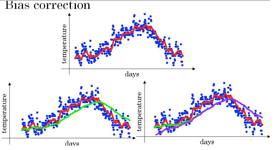
Let's see how that works. In a previous section, you saw this figure for beta = 0.9. This figure for beta = 0.98. But it turns out that if you implement the formula as written here, you won't actually get the green curve when, say, beta = 0.98.

You actually get the purple curve here.

And you notice that the purple curve starts off really low.

So let's see how it affects that.

When you're implementing a moving average, you initialize it with v0 = 0, and then v1 = 0.98 V0 + 0.02 theta 1.

But V0 is equal to 0 so that term just goes away. So V1 is just 0.02 times theta 1. \( V_0 = 0 \\ V_1 = 0.98V_0 + 0.02\theta_1 \\ V_2 = 0.98V_1 + 0.02\theta_2 \\ V_3 = 0.98V_2 + 0.02\theta_3 \\ . \\ . \\ . \\ . \\ V_t = 0.98V_{t-1} + 0.02\theta_t \)

So that's why if the first day's temperature is, say 40 degrees Fahrenheit, then v1 will be 0.02 times 40, which is 8.

So you get a much lower value down here. So it's not a very good estimate of the first day's temperature.

So it turns out that there is a way to modify this estimate that makes it much better, that makes it more accurate, especially during this initial phase of your estimate.

Which is that, instead of taking V_t, take V_t divided by 1- β to the power of t where t is the current data here on. \( V_t → \frac{V_t}{1 - \beta^t} \) So let's take a concrete example.

When t = 2, \( \frac{1}{1 - \beta^t} \) is 0.0396.

And so your estimate of the tempature on day 2 becomes \( \frac{V_2}{1 - \beta^2} = 0.98V_1 + 0.02\theta_2 \\ V_2 = \frac{0.98V_1 + 0.02\theta_2}{0.0396} \\ \) .

Andso this becomes a weighted average of theta 1 and theta 2 and this removes this bias. So you notice that as t becomes large, β^t will approach 0 which is why when t is large enough, the bias correction makes almost no difference.

This is why when t is large, the purple line and the green line pretty much overlap.

But during this initial phase of learning when you're still warming up your estimates when the bias correction can help you to obtain a better estimate of this temperature.

And it is this bias correction that helps you go from the purple line to the green line.

So in machine learning, for most implementations of the exponential weighted average, people don't often bother to implement bias corrections.

Because most people would rather just wait that initial period and have a slightly more biased estimate and go from there.

But if you are concerned about the bias during this initial phase, while your exponentially weighted moving average is still warming up.

Then bias correction can help you get a better estimate early on. So you now know how to implement exponentially weighted moving averages.

Let's go on and use this to build some better optimization algorithms.