You've seen how using momentum can speed up gradient descent. There's another algorithm called RMSprop, which stands for root mean square prop, that can also speed up gradient descent.

Let's see how it works.

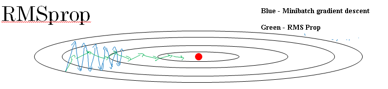
Recall our example from before, that if you implement gradient descent, you can end up with huge oscillations in the vertical direction, even while it's trying to make progress in the horizontal direction.

In order to provide intuition for this example, let's say that the vertical axis is the parameter b and horizontal axis is the parameter w.

And so, you want to slow down the learning in the b direction, or in the vertical direction. And speed up learning, or at least not slow it down in the horizontal direction.

So this is what the RMSprop algorithm does to accomplish this. On iteration t, it will compute as usual the derivative dW, db on the current mini-batch.

 On iteration t:
    Computing dW, dB on current mini batch
    SdW = βSdW + (1 - β)dW2
    SdB = βSdB + (1 - β)dB2
    
    W := W - α dW / (√SdW  )
    b := b - α dB / (√SdB )

So I was going to keep this exponentially weighted average. Instead of VdW, I'm going to use the new notation SdW. So SdW is equal to beta times their previous value + 1- beta times dW squared.

Sometimes we use dW as dW squared.

So for clarity, this squaring operation is an element-wise squaring operation. So what this is doing is really keeping an exponentially weighted average of the squares of the derivatives.

And similarly, we also have Sdb equals beta Sdb + 1- beta, db squared.

And again, the squaring is an element-wise operation.

Next, RMSprop then updates the parameters as follows. W gets updated as W minus the learning rate, and whereas previously we had alpha times dW, now it's dW divided by square root of SdW.

And b gets updated as b minus the learning rate times, instead of just the gradient, this is also divided by, now divided by Sdb.

So let's gain some intuition about how this works.

Recall that in the horizontal direction or in this example, in the W direction we want learning to go pretty fast.

Whereas in the vertical direction or in this example in the b direction, we want to slow down all the oscillations into the vertical direction.

So with this terms SdW an Sdb, what we're hoping is that SdW will be relatively small, so that here we're dividing by relatively small number.

Whereas Sdb will be relatively large, so that here we're dividing relatively large number in order to slow down the updates on a vertical dimension.

And indeed if you look at the derivatives, these derivatives are much larger in the vertical direction than in the horizontal direction.

So the slope is very large in the b direction. So with derivatives like this, this is a very large db and a relatively small dw.

Because the function is sloped much more steeply in the vertical direction than as in the b direction, than in the w direction, than in horizontal direction.

And so, db squared will be relatively large. So Sdb will relatively large, whereas compared to that dW will be smaller, or dW squared will be smaller, and so SdW will be smaller.

So the net effect of this is that your updates in the vertical direction are divided by a much larger number, and so that helps damp out the oscillations.

Whereas the updates in the horizontal direction are divided by a smaller number. So the net impact of using RMSprop is that your updates will end up looking more like this red line in the image above.

That your updates in the, Vertical direction and then horizontal direction you can keep going.

And one effect of this is also that you can therefore use a larger learning rate alpha, and get faster learning without diverging in the vertical direction.

Now just for the sake of clarity, I've been calling the vertical and horizontal directions b and w, just to illustrate this.

In the next section, we're actually going to combine RMSprop together with momentum.

So rather than using the hyperparameter beta, which we had used for momentum, we are going to call this hyperparameter beta 2 just to not clash.

The same hyperparameter for both momentum and for RMSprop.

And also to make sure that your algorithm doesn't divide by 0.

What if square root of SdW, right, is very close to 0. Then things could blow up. Just to ensure numerical stability, when you implement this in practice you add a very, very small epsilon to the denominator.

It doesn't really matter what epsilon is used. 10^-8 would be a reasonable default, but this just ensures slightly greater numerical stability that for numerical round off or whatever reason, that you don't end up dividing by a very, very small number.

 On iteration t:
    Computing dW, dB on current mini batch
    SdW = βSdW + (1 - β)dW2
    SdB = βSdB + (1 - β)dB2
    
    W := W - α dW / (√SdW    + ε)
    b := b - α dB / (√SdB  + ε)