One of the things that might help speed up your learning algorithm, is to slowly reduce your learning rate over time.

We call this learning rate decay.

Let's see how you can implement this.

Let's start with an example of why you might want to implement learning rate decay.

Suppose you're implementing mini-batch gradient descent, with a reasonably small mini-batch. Maybe a mini-batch has just 64, 128 examples.

Then as you iterate, your steps will be a little bit noisy.

And it will tend towards this minimum, but it won't exactly converge.

But your algorithm might just end up wandering around, and never really converge, because you're using some fixed value for alpha.

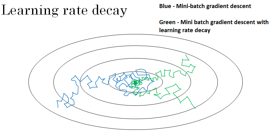
And there's just some noise in your different mini-batches.

But if you were to slowly reduce your learning rate alpha, then during the initial phases, while your learning rate alpha is still large, you can still have relatively fast learning.

But then as alpha gets smaller, your steps you take will be slower and smaller.

And so you end up oscillating in a tighter region around this minimum, rather than wandering far away, even as training goes on and on.

So the intuition behind slowly reducing alpha, is that maybe during the initial steps of learning, you could afford to take much bigger steps.

But then as learning approaches converges, then having a slower learning rate allows you to take smaller steps. So here's how you can implement learning rate decay.

Recall that one epoch is one pass, So if you have a training set then the first pass through the training set is called the first epoch, and then the second pass is the second epoch, and so on.

So one thing you could do, is set your learning rate alpha \( \alpha = \frac{1}{1 + decay_rate * epoch_number} \alpha_0 \)

. And this is going to be times some initial learning rate \( \alpha_0 \). Note that the decay rate here becomes another hyper-parameter, which you might need to tune.

Hence, as a function of your epoch number, your learning rate gradually decreases, right, according to this formula up on top.

So if you wish to use learning rate decay, what you can do, is try a variety of values of both hyper-parameter \( \alpha_0 \). As well as this decay rate hyper-parameter, and then try to find the value that works well.

Other than this formula for learning rate decay, there are a few other ways that people use.

For example, this is called exponential decay. Where alpha is \( \alpha = 0.95^{epoch_num} * \alpha_0 \). So this will exponentially quickly decay your learning rate.

Other formulas that people use are things like alpha \( \alpha = \frac{k}{\sqrt{epoch_num}} * \alpha_0 \). Or \( \alpha = \frac{k}{\sqrt{t}} * \alpha_0 \) where t is the mini batch size.

And sometimes you also see people use a learning rate that decreases in discrete steps. Wherefore some number of steps, you have some learning rate, and then after a while you decrease it by one half. After a while by one half. After a while by one half. And so this is a discrete staircase.

So so far, we've talked about using some formula to govern how alpha, the learning rate, changes over time. One other thing that people sometimes do, is manual decay.

And so if you're training just one model at a time, and if your model takes many hours, or even many days to train. What some people will do, is just watch your model as it's training over a large number of days.

And then manually say, it looks like the learning rate slowed down, I'm going to decrease alpha a little bit. Of course this works, this manually controlling alpha, really tuning alpha by hand, hour by hour, or day by day.

This works only if you're training only a small number of models, but sometimes people do that as well.