In the rise of deep learning, one of the most important ideas has been an algorithm called batch normalization, created by two researchers, Sergey Ioffe and Christian Szegedy.

Batch normalization makes your hyperparameter search problem much easier, makes your neural network much more robust.

It will also enable you to much more easily train even very deep networks.

Let's see how batch normalization works.

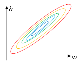
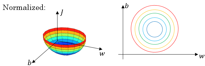
When training a model, such as logistic regression, you might remember that normalizing the input features can speed up learnings

And we saw in an earlier section how this can turn the contours of your learning problem from something that might be very elongated to something that is more round, and easier for an algorithm like gradient descent to optimize.

So this works, in terms of normalizing the input feature values to a neural network, alter the regression.

Now, how about a deeper model? You have not just input features x, but in this layer you have activations \( a^{[1]} \), in this layer, you have activations \( a^{[2]} \) and so on.

So if you want to train the parameters, say \( w^{[3]} \), \( b^{[3]} \), then wouldn't it be nice if you can normalize the mean and variance of \( a^{[2]} \) to make the training of \( w^{[3]} \), \( b^{[3]} \) more efficient?

In the case of logistic regression, we saw how normalizing \(x_1, x_2, x_3 \) (features of the input data) maybe helps you train w and b more efficiently.

So here, the question is, for any hidden layer, can we normalize, The values of a so as to train \( w^{[3]} \), \( b^{[3]} \) faste

Since \( a^{[2]} \) is the input to the next layer, that therefore affects your training of \( w^{[3]} \) and \( b^{[3]} \).

So this is what batch norm does.

Although technically, we'll actually normalize the values of not \( a^{[2]} \) but \( z^{[2]} \). There are some debates in the deep learning literature about whether you should normalize the value before the activation function, so \( z^{[2]} \), or whether you should normalize the value after applying the activation function, \( a^{[2]} \).

In practice, normalizing \( z^{[2]} \) is done much more often.

So that's the version presented here and what I would recommend you use as a default choice.

So here is how you will implement batch norm.

Given some intermediate values, In your neural net, Let's say that you have some hidden unit values \( z^{[1]} \) up to \( z^{[m]} \), then batch norm is computed as follows;

\( \mu = \frac{1}{m} \sum_{i} z^{[i]}\\ \sigma^2 = \frac{1}{m} \sum_{i} (z^{[i]} - \mu) \\ z^{[i]}_{norm} = \frac{(z^{[i]} - \mu)}{\sqrt{\sigma^2 + \epsilon}} \)

For numerical stability, we usually add epsilon to the denominator like that just in case sigma squared turns out to be zero in some estimate.

And so now we've taken these values z and normalized them to have mean 0 and standard unit variance. So every component of z has mean 0 and variance 1. But we don't want the hidden units to always have mean 0 and variance 1.

Maybe it makes sense for hidden units to have a different distribution, so what we'll do instead is compute

\( \widetilde{z}^{[i]} = \gamma z^{[i]}_{norm} + \beta \)

And here, gamma and beta are learnable parameters of your model.

So we're using gradient descent, or some other algorithm, like the gradient descent with momentum, or RMS prop or ADAM, you would update the parameters gamma and beta, just as you would update the weights of your neural network.

Now, notice that the effect of gamma and beta is that it allows you to set the mean of \( \widetilde{z}^{[i]} \) to be whatever you want it to be.

So the intuition I hope you'll take away from this is that we saw how normalizing the input features x can help learning in a neural network. And what batch norm does is it applies that normalization process not just to the input layer, but to the values even deep in some hidden layer in the neural network. So it will apply this type of normalization to normalize the mean and variance of some of your hidden units' values, z. But one difference between the training input and these hidden unit values is you might not want your hidden unit values be forced to have mean 0 and variance 1.

For example, if you have a sigmoid activation function,you might want them to have a larger variance or have a mean that's different than 0, in order to better take advantage of the nonlinearity of the sigmoid function rather than have all your values be in just this linear regime.

So that's why with the parameters gamma and beta, you can now make sure that your \( z^{[i]} \) values have the range of values that you want.

But what it does really is it then shows that your hidden units have standardized mean and variance, where the mean and variance are controlled by two explicit parameters gamma and beta which the learning algorithm can set to whatever it wants.

So I hope that gives you a sense of the mechanics of how to implement batch norm, at least for a single layer in the neural network. In the next video, I'm going to show you how to fit batch norm into a neural network, even a deep neural network, and how to make it work for the many different layers of a neural network.

And after that, we'll get some more intuition about why batch norm could help you train your neural network. So in case why it works still seems a little bit mysterious, stay with me, and I think in two sections from now we'll really make that clearer.

So you have seen the equations for how to invent Batch Norm for maybe a single hidden layer.

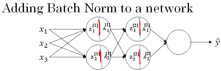
Let's see how it fits into the training of a deep network. So, let's say you have a neural network like this, you've seen me say before that you can view each of the unit as computing two things.

First, it computes Z and then it applies the activation function to compute A. And so we can think of each of these circles as representing a two step computation.

And similarly for the next layer, that is \(Z^{[2]}_1 \), and \( A^{[2]}_1 \), and so on. So, if you were not applying Batch Norm, you would have an input X fit into the first hidden layer, and then first compute \(Z^{[1]} \), and this is governed by the parameters \( W^{[1]} \) and \( B^{[1]} \).

And then ordinarily, you would fit \(Z^{[1]} \) into the activation function to compute \( A^{[1]} \). But what would do in Batch Norm is take this value \(Z^{[1]} \), and apply Batch Norm, sometimes abbreviated BN to it, and that's going to be governed by parameters, \( \beta_1, \gamma_1 \), and this will give you this new normalize value \(Z^{[1]} \).

And then you fit that to the activation function to get \( A^{[1]} \), which is \( g^{[1]}(\widetilde{Z}^{[1]}) \).

Now, you've done the computation for the first layer, where this Batch Norms that really occurs in between the computation from Z and A.

Next, you take this value \( A^{[1]} \) and use it to compute \( Z^{[2]} \), and so this is now governed by \( W^{[2]} \), \( B^{[2]} \). And similar to what you did for the first layer, you would take \( Z^{[2]} \) and apply it through Batch Norm, and we abbreviate it to BN now.

This is governed by Batch Norm parameters specific to the next layer.

So \( \beta_2, \gamma_2 \), and now this gives you \( \widetilde{Z}^{[2]} \), and you use that to compute \( A^{[2]} \) by applying the activation function, and so on. So once again, the Batch Norms that happens between computing Z and computing A.

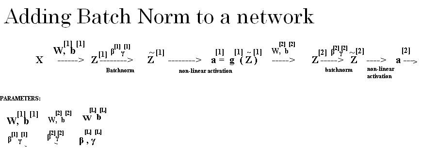
And the intuition is that, instead of using the un-normalized value Z, you can use the normalized value \( \widetilde{Z}^{[1]} \), that's the first layer.

The second layer as well, instead of using the un-normalized value Z2, you can use the mean and variance normalized values \( \widetilde{Z}^{[2]} \) (Z tilde 2). So the parameters of your network are going to be \( W^{[1]} \), \( B^{[1]} \).

It turns out we'll get rid of the parameters but we'll see why in the next section.

But for now, imagine the parameters are the usual \( W^{[1]} \), \( B^{[1]} \), ..., \( W^{[L]} \), \( B^{[L]} \) and we have added to this new network, additional parameters \( \beta_1, \gamma_1, \beta_2, \gamma_2 \), and so on, for each layer in which you are applying Batch Norm.

For clarity, note that these Betas here, these have nothing to do with the hyperparameter beta that we had for momentum over the computing the various exponentially weighted averages.

The \( \beta_1, \beta_2 \), and so on, that Batch Norm tries to learn is a different Beta than the hyperparameter Beta used in momentum and the Adam and RMSprop algorithms.

So now that these are the new parameters of your algorithm, you would then use an optimization you want, such as gradient descent in order to implement it.

For example, you might compute \( d\beta^{[L]}\) for a given layer, and then update the parameters Beta, gets updated as Beta minus learning rate times \( d\beta^{[L]}\).

\( \text{for t = 1,...., num_of_mini_batches}\\ \text{Compute forward propagation on} X^{t} \text{In hidden layers compute} \widetilde{Z}^{[L]} from Z^{[L]}\\ \text{Use back propagation to compute} dW^{[L]}, db^{[L]}, d\beta^{[L]}, d\gamma^{[L]}\\ \text{Update parameters:}\\ W^{[L]} = W^{[L]} - \alpha * dW^{[L]}\\ b^{[L]} = b^{[L]} - \alpha * db^{[L]}\\ \beta^{[L]} = \beta^{[L]} - \alpha * d\beta^{[L]}\\ \gamma^{[L]} = \gamma^{[L]} - \alpha * d\gamma^{[L]}\\ \)

And you can also use Adam or RMSprop or momentum in order to update the parameters Beta and Gamma, not just gradient descent.

And even though in the previous section, I had explained what the Batch Norm operation does, computes mean and variances and subtracts and divides by them.

If they are using a Deep Learning Programming Framework, usually you won't have to implement the Batch Norm step on Batch Norm layer yourself.

Now, so far, we've talked about Batch Norm as if you were training on your entire training site at the time as if you are using Batch gradient descent.

In practice, Batch Norm is usually applied with mini-batches of your training set. So the way you actually apply Batch Norm is you take your first mini-batch and compute \(Z^{[1]} \).

Same as we did on the previous section using the parameters \( W^{[1]} \), \( B^{[1]} \) and then you take just this mini-batch and computer mean and variance of the \(Z^{[1]} \) on just this mini batch and then Batch Norm would subtract by the mean and divide by the standard deviation and then re-scale by \( \beta_1, \gamma_1 \), to give you \(Z^{[1]} \), and all this is on the first mini-batch, then you apply the activation function to get \( A^{[1]} \), and then you compute \(Z^{[2]} \) using \( W^{[2]} \), \( B^{[2]} \), and so on.

So you do all this in order to perform one step of gradient descent on the first mini-batch X^{1} and then goes to the second mini-batch X^{2}, and you do something similar where you will now compute \(Z^{[1]} \) on the second mini-batch and then use Batch Norm to compute \( \widetilde{Z}^{[1]} \).

And so here in this Batch Norm step, You would be normalizing \( \widetilde{Z}^{[1]} \) using just the data in your second mini-batch, so does Batch Norm step here. Let's look at the examples in your second mini-batch, computing the mean and variances of the \(Z^{[1]} \)'s on just that mini-batch and re-scaling by Beta and Gamma to get \( \widetilde{Z}^{[1]} \), and so on.

And you do this with a third mini-batch, and keep training. Now, there's one detail to the parameterization that I want to clean up, which is previously, I said that the parameters was \( W^{[L]} \), \( B^{[L]} \), for each layer as well as \( \beta_L, \gamma_L \).

Now notice that the way Z was computed is as follows, \( Z^{[L]} = W^{[L]} * A^{[L-1]} + B^{[L]} \).

But what Batch Norm does, is it is going to look at the mini-batch and normalize \( Z^{[L]} \) to first of mean 0 and standard variance, and then a rescale by Beta and Gamma.

But what that means is that, whatever is the value of \( B^{[L]} \) is actually going to just get subtracted out, because during that Batch Normalization step, you are going to compute the means of the \( Z^{[L]} \)'s and subtract the mean.

And so adding any constant to all of the examples in the mini-batch, it doesn't change anything. Because any constant you add will get cancelled out by the mean subtractions step.

So, if you're using Batch Norm, you can actually eliminate that parameter, or if you want, think of it as setting it permanently to 0.

So then the parameterization becomes \( Z^{[L]} = W^{[L]} * A^{[L-1]} \), And then you compute \( Z^{[L]}_{norm} \), and we compute \( \widetilde{Z}^{[L]} = \gamma_L Z^{[L]} + \beta_L \) Z tilde = Gamma ZL + Beta, you end up using this parameter \( \beta_L \) in order to decide whats that mean of \( \widetilde{Z}^{[L]} \) Z tilde L. Which is why guess post in this layer.

So just to recap, because Batch Norm zeroes out the mean of these \( Z^{[L]} \) values in the layer, there's no point having this parameter \( B^{[L]} \) , and so you must get rid of it, and instead is sort of replaced by \( \beta_L \), which is a parameter that controls that ends up affecting the shift or the biased terms.

Finally, remember that the dimension of \( Z^{[L]} \) , because if you're doing this on one example, it's going to be \( N^{[L]} by 1 \) , and so \( B^{[L]} \), a dimension, \( N^{[L]} by 1 \), if \( N^{[L]} \) was the number of hidden units in layer L.

And so the dimension of \( \beta_L \) and \( \gamma_L \) is also going to be \( N^{[L]} by 1 \) because that's the number of hidden units you have. You have \( N^{[L]} \) hidden units, and so \( \beta_L \) and \( \gamma_L \) are used to scale the mean and variance of each of the hidden units to whatever the network wants to set them to.

So, let's pull all together and describe how you can implement gradient descent using Batch Norm. Assuming you're using mini-batch gradient descent, it rates for T = 1 to the number of many batches.

You would implement forward prop on mini-batch X^T and doing forward prop in each hidden layer, use Batch Norm to replace \( Z^{[L]} \) with \( \widetilde{Z}^{[L]} \) Z tilde L.

And so then it shows that within that mini-batch, the value Z end up with some normalized mean and variance and the values and the version of the normalized mean that and variance is \( \widetilde{Z}^{[L]} \) Z tilde L. And then, you use back prop to compute DW, DB, for all the values of L, D Beta, D Gamma.

Although, technically, since you have got to get rid of B, this actually now goes away.

And then finally, you update the parameters. So, W gets updated as W minus the learning rate times, as usual, Beta gets updated as Beta minus learning rate times DB, and similarly for Gamma.

And if you have computed the gradient as follows, you could use gradient descent. That's what I've written down here, but this also works with gradient descent with momentum, or RMSprop, or Adam.

Where instead of taking this gradient descent update, mini-batch you could use the updates given by these other algorithms as we discussed in the previous sections.

Some of these other optimization algorithms as well can be used to update the parameters Beta and Gamma that Batch Norm added to algorithm.

So, I hope that gives you a sense of how you could implement Batch Norm from scratch if you wanted to.

If you're using one of the Deep Learning Programming frameworks , hopefully you can just call someone else's implementation in the Programming framework which will make using Batch Norm much easier.

Now, in case Batch Norm still seems a little bit mysterious if you're still not quite sure why it speeds up training so dramatically, let's go to the next section and talk more about why Batch Norm really works and what it is really doing.