So far, the classification examples we've talked about have used binary classification, where you had two possible labels, 0 or 1. Is it a cat, is it not a cat?

What if we have multiple possible classes? There's a generalization of logistic regression called Softmax regression.

In this you make predictions where you're trying to recognize one of C or one of multiple classes, rather than just recognize two classes.

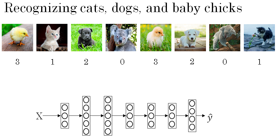
Let's say that instead of just recognizing cats you want to recognize cats, dogs, and baby chicks. So I'm going to call cats class 1, dogs class 2, baby chicks class 3.

And if none of the above, then there's an other or a none of the above class, which I'm going to call class 0.

So below is an example of the images and the classes they belong to. That's a picture of a baby chick, so the class is 3. Cats is class 1, dog is class 2, and a koala, so that's none of the above, so that is class 0, class 3 and so on.

So the notation we're going to use is, capital C to denote the number of classes you're trying to categorize your inputs into. And in this case, you have four possible classes, including the other or the none of the above class.

So when you have four classes, the numbers indexing your classes would be 0 through capital C minus one. So in other words, that would be zero, one, two or three.

In this case, we're going to build a new X -> Y, where the upper layer has four, or in this case the variable capital alphabet C upward units.

So N, the number of units upper layer which is layer L is going to equal to 4 or in general this is going to equal to C. And what we want is for the number of units in the upper layer to tell us what is the probability of each of these four classes.

So the first node is supposed to output the probability that the image is of a cat given the input x. The second node will output probability that image is a dog. The third node will output the probability that image contains a baby chick given the input x. Fourth node will give the probability of the image having none of the above clases given input x.

So here, the output labels \( \hat{y} \) (y hat) is going to be a four by one dimensional vector, because it now has to output four numbers, giving you these four probabilities.

And because probabilities should sum to one, the four numbers in the output \( \hat{y} \) (y hat), they should sum to one.

The standard model for getting your network to do this uses what's called a Softmax layer, and the output layer in order to generate these outputs.

So in the final layer of the neural network, you are going to compute as usual the linear part of the layers. So \( Z^{[L]} \), that's the z variable for the final layer.

So remember this last layer of the neural network is layer capital L. So as usual you compute that as \( Z^{[L]} = {W^{[L]}}^T A^{[L-1]} + b^{[L]} \) which i weights of the layer times the activation of the previous layer plus the biases for that final layer.

Now having computed \( Z^{[L]} \), you now need to apply what's called the Softmax activation function.

So that activation function is a bit unusual for the Softmax layer, but this is what it does.

First, we're going to compute a temporary variable, which we're going to call t, which is \( e^{Z^{[L]}} \). So this is a part performed element-wise. So \( Z^{[L]} \) here, in our example, \( Z^{[L]} \) is going to be four by one vector. This is a four dimensional vector.

So t Itself \( t = e^{Z^{[L]}} \), that's an element wise exponentiation. T will also be a 4*1 dimensional vector.

Then the output \( A^{[L]} \), is going to be basically the vector t will normalized to sum to 1.

So \( A^{[L]} \) is going to be \( \frac{e^{Z^{[L]}}}{\sum_{j=1}^{4} t_i } \), because we have four classes of t (cat, dog, baby chick, none).

So in other words we're saying that \( A^{[L]} \) is also a four by one vector, and the i element of this four dimensional vector.

Let's write that, \( A^{[L]}_i = \frac{t_i}{\sum_{j=1}^{4} t_i } \)

In case this math isn't clear, we'll do an example in a minute that will make this clearer.

Let's say that your computer \( Z^{[L]} \), and \( Z^{[L]} \) is a four dimensional vector, let's say is 5, 2, -1, 3 \( Z^{[L]} = \begin{bmatrix} 5 \\ 2 \\ -1 \\ 3 \end{bmatrix} \). What we're going to do is use this element-wise exponentiation to compute this vector t.

So t is going to be e to the 5, e to the 2, e to the -1, e to the 3 i.e. \( t = \begin{bmatrix} e^5 \\ e^2 \\ e^{-1} \\ e^3 \end{bmatrix} \). And if you plug that in the calculator, these are the values you get \( t = \begin{bmatrix} 148.4 \\ 7.4 \\ 0.4 \\ 20.1 \end{bmatrix} \) .

And so, the way we go from the vector t to the vector \( A^{[L]} \) is just to normalize these entries to sum to one.

So if you sum up the elements of t, if you just add up those 4 numbers you get 176.3 \( \sum_{j=1}^{4} t_i = 176.3 \). So finally, \( A^{[L]} \) is just going to be this vector t, as a vector, divided by 176.3.

So for example \( A^{[L]} = \begin{bmatrix} 148.4/176.3 \\ 7.4/176.3 \\ 0.4/176.3 \\ 20.1/176.3 \end{bmatrix} \), the first node here, this will output e to the 5 divided by 176.3. And that turns out to be 0.842. So saying that, for this image, if this is the value of z you get, the chance of it being called zero is 84.2%. And then the next nodes outputs e squared over 176.3, that turns out to be 0.042, so this is 4.2% chance \( A^{[L]} = \begin{bmatrix} 0.842 \\ 0.042 \\ 0.002 \\ 0.114 \end{bmatrix} \).

So it is 11.4% chance that this is class number three, which is the baby C class, right? So there's a chance of it being class zero, class one, class two, class three. So the output of the neural network \( A^{[L]} \), this is also y hat.

This is a 4 by 1 vector where the elements of this 4 by 1 vector are going to be these four numbers. Then we just compute it. So this algorithm takes the vector \( Z^{[L]} \) and is four probabilities that sum to 1.

And if we summarize what we just did to math from \( Z^{[L]} \) to \( A^{[L]} \), this whole computation confusing exponentiation to get this temporary variable t and then normalizing, we can summarize this into a Softmax activation function and say aL equals the activation function g applied to the vector \( Z^{[L]} \).

The unusual thing about this particular activation function is that, this activation function g, it takes a input a 4 by 1 vector and it outputs a 4 by 1 vector.

So previously, our activation functions used to take in a single row value input. So for example, the sigmoid and the value activation functions input the real number and output a real number.

The unusual thing about the Softmax activation function is, because it needs to normalized across the different possible outputs, and needs to take a vector and puts in outputs of vector. So one of the things that a Softmax cross layer can represent, I'm going to show you some examples where you have inputs \( x_1, x_2 \). And these feed directly to a Softmax layer that has three or four, or more output nodes that then output \( \hat{y} \) y hat.

So I'm going to show you a new network with no hidden layer, and all it does is compute \( Z^{[1]} = {W^{[1]}}^T X + b^{[1]} \) i.e. z1 equals w1 times the input x plus b. And then the output \( A^{[1]} \), or \( \hat{y} \) y hat is just the Softmax activation function applied to \( Z^{[1]} \).

So in this neural network with no hidden layers, it should give you a sense of the types of things a Softmax function can represent. So here's one example with just raw inputs x1 and x2.

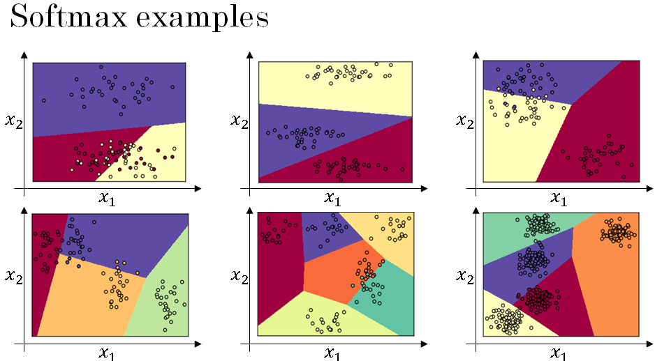
A Softmax layer with C equals 3 upper classes can represent the type of decision boundaries shown below. Notice this kind of several linear decision boundaries, but this allows it to separate out the data into three classes. And in this diagram, what we did was we actually took the training set that's kind of shown in this figure and train the Softmax cross fire with the upper labels on the data.

And then the color on the plot above shows fresh holding the upward of the Softmax classifier, and coloring in the input base on which one of the three outputs have the highest probability.

So we can maybe we kind of see that this is like a generalization of logistic regression with sort of linear decision boundaries, but with more than two classes class 0, 1, the class could be 0, 1, or 2. Here's another example of the decision boundary that a Softmax classifier represents when three normal datasets with three classes.

And the plot above has intuition that the decision boundary between any two classes will be more linear. That's why you see for example that decision boundary between the yellow and the various classes, that's the linear boundary where the purple and red linear in boundary between the purple and yellow and other linear decision boundary. But able to use these different linear functions in order to separate the space into three classes.

Let's look at the plot above some examples with more classes. So it's an example with C equals 4, so that the green class and Softmax can continue to represent these types of linear decision boundaries between multiple classes. So here's one more example with C equals 5 classes, and here's one in the plot above last example with C equals 6.

So the plot above shows the type of things the Softmax classifier can do when there is no hidden layer of class, even much deeper neural network with x and then some hidden units, and then more hidden units, and so on. Then you can learn even more complex non-linear decision boundaries to separate out multiple different classes.

So I hope this gives you a sense of what a Softmax layer or the Softmax activation function in the neural network can do. In the next section, let's take a look at how you can train a neural network that uses a Softmax layer.

In the last section, you learned about the softmax activation function.

In this section, you deepen your understanding of softmax classification, and also learn how the training model that uses a softmax layer.

Recallour earlier example where the output layer computes \( Z^{[L]} \) as follows.

So we have four classes, c = 4 then z[L] can be (4,1) dimensional vector \( Z^{[L]} = \begin{bmatrix} 5 \\ 2 \\ -1 \\ 3 \end{bmatrix} \) and we said we compute t \( t = e^{Z^{[L]}} \) which is this temporary variable that performs element y's exponentiation \( t = \begin{bmatrix} e^5 \\ e^2 \\ e^{-1} \\ e^3 \end{bmatrix} \) .

And then finally, if the activation function for your output layer, \( g^{[L]} \) is the softmax activation function, then your outputs will be this \( t = \begin{bmatrix} \frac{e^5}{e^5 + e^2 + e^{-1} + e^3} \\ \frac{e^2}{e^5 + e^2 + e^{-1} + e^3} \\ \frac{e^{-1}}{e^5 + e^2 + e^{-1} + e^3} \\ \frac{e^3}{e^5 + e^2 + e^{-1} + e^3} \end{bmatrix} \).

It's basically taking the temporarily variable t and normalizing it to sum to 1.

So this then becomes \( A^{[L]} \) . So you notice that in the z vector, the biggest element was 5, and the biggest probability ends up being this first probability.

The name softmax comes from contrasting it to what's called a hard max which would have taken the vector Z and converted it to this vector \( t = \begin{bmatrix} 1 \\ 0 \\ 0 \\ 0 \end{bmatrix} \).

So hard max function will look at the elements of Z and just put a 1 in the position of the biggest element of Z and then 0s everywhere else.

And so this is a hard max where the biggest element gets a output of 1 and everything else gets an output of 0.

Whereas in contrast, a softmax is a more gentle mapping from Z to these probabilities.

And one thing I didn't really show but had alluded to is that softmax regression or the softmax identification function generalizes the logistic activation function to C classes rather than just two classes.

And it turns out that if C = 2, then softmax with C = 2 essentially reduces to logistic regression.

Now let's look at how you would actually train a neural network with a softmax output layer. So in particular, let's define the loss functions you use to train your neural network.

Let's see of an example in your training set where the target output, the ground true label is 0 1 0 0 i.e. \( y = \begin{bmatrix} 0 \\ 1 \\ 0 \\ 0 \end{bmatrix} \).

So the example from the previous section, this means that this is an image of a cat because it falls into Class 1.

And now let's say that your neural network is currently outputting \( \hat{y} = \begin{bmatrix} 0.3 \\ 0.2 \\ 0.1 \\ 0.4 \end{bmatrix} \).

So the neural network's not doing very well in this example because this is actually a cat and assigned only a 20% chance that this is a cat. So didn't do very well in this example.

So what's the loss function you would want to use to train this neural network? In softmax classification, its shown as \( L(y, \hat{y}) = - \sum_{j=1}^{4} y_j log \hat{y_j} \).

So let's look at our single example above to better understand what happens. Notice that in this example, y1 = y3 = y4 = 0 because those are 0s and only y2 = 1 i.e. \( y = \begin{bmatrix} 0 \\ 1 \\ 0 \\ 0 \end{bmatrix} \). So if you look at this summation of loss function, all of the terms with 0 values of yj were equal to 0.

And the only term you're left with is \( -y_2 log (\hat{y_2}) \) , because we use sum over the indices of j, all the terms will end up 0, except when j is equal to 2. And because y2 = 1, this is just \( - log (\hat{y_2}) \).

So what this means is that, if your learning algorithm is trying to make \( - log (\hat{y_2}) \) small because you use gradient descent to try to reduce the loss on your training set. Then the only way to make \( - log (\hat{y_2}) \) small is to make this small. And the only way to do that is to make \( \hat{y_2} \) as big as possible.

And these are probabilities, so they can never be bigger than 1. But this kind of makes sense because x for this example is the picture of a cat, then you want that output probability to be as big as possible.

So more generally, what this loss function does is it looks at whatever is the ground true class in your training set, and it tries to make the corresponding probability of that class as high as possible.

Finally, let's take a look at how you'd implement gradient descent when you have a softmax output layer.

So this output layer will compute \( Z^{[L]} \) which is C by 1 in our example, 4 by 1 and then you apply the softmax function to get \( A^{[L]} \) or \( \hat{y} \).

For the backward propagation step you can refer to the programming assignments with this section. But if you are using a programming framework such as Tensorflow, the framework handles backward propagation step.