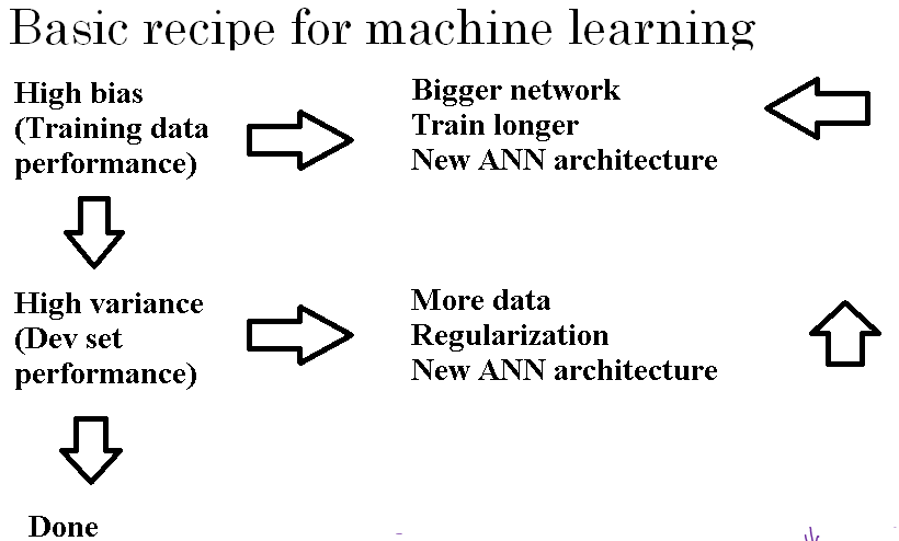
If you suspect your neural network is over fitting your data. That is you have a high variance problem, one of the first things you should try per probably regularization.

The other way to address high variance, is to get more training data that's also quite reliable.

But you can't always get more training data, or it could be expensive to get more data.

But adding regularization will often help to prevent overfitting, or to reduce the errors in your network. So let's see how regularization works.

Recall that for logistic regression, you try to minimize the cost function J, which is defined as the cost function given below.

\( J(w,b) = − \frac{1}{m} \sum_{i = 1}^{m} L(\hat{y}^{(i)}, y^{(i)}) = − \frac{1}{m} \sum_{i = 1}^{m} [y^{(i)}log(\hat{y}^{(i)})−(1−y^{(i)})log(1−\hat{y}^{(i)}) ] \)

Sum of your training examples of the losses of the individual predictions in the different examples, where you recall that w and b in the logistic regression, are the parameters.

So w is an n_x-dimensional (n_x number of features) parameter vector, and b is a real number. And so to add regularization to the logistic regression you add lambda, which is called the regularization parameter.

Usually L2 regularization is applied to regularize the model. L2 regularization is the defined as \( \frac{\lambda}{2m} ||w||^2_2 \).

This is read as lambda/2m times the norm of w squared. So here, the norm of w squared is just written w transpose w ( \( ||w||^2_2 = \sum_{j = 1}^{n_x} w_j^2 \) ), it's just a square Euclidean norm of the vector w.

Now, why do you regularize just the parameter w? Why don't we add something here about b as well? \( \frac{\lambda}{2m} ||b||^2_2 \)

In practice, you could do this, but we usually just omit this.

Because if you look at your parameters, w is usually a pretty high dimensional parameter vector, especially with a high variance problem.

Maybe w just has a lot of parameters, so you aren't fitting all the parameters well, whereas b is just a single number.

So almost all the parameters are in w rather b. And if you add this last term, in practice, it won't make much of a difference, because b is just one parameter over a very large number of parameters.

In practice, we usually just don't bother to include it. But you can if you want.

So L2 regularization is the most common type of regularization.

You might have also heard of some people talk about L1 regularization. And that's when you add, instead of this L2 norm, add a term that is lambda/m of sum over of this i.e \( \frac{\lambda}{2m} ||w||_1 \).

And this is also called the L1 norm of the parameter vector w

The last detail - Lambda is called the regularization parameter.

And usually, you set this using your development set, or using cross validation.

Regularization helps prevent over fitting. So lambda is another hyper parameter that you might have to tune. Note that, for the programming exercises, lambda is a reserved keyword in the Python programming language. So in the programming exercise, we'll have lambd.

This is how you implement L2 regularization for logistic regression.

In a neural network, you have a cost function that's a function of all of your parameters, \( w^{[1]}, b^{[1]} \) through \( w^{[L]}, b^{[L]} \), where capital L is the number of layers in your neural network.

And so the cost function of this is given below, sum of the losses, summed over your m training examples.

\( J( w^{[1]}, b^{[1]} , .... , w^{[L]}, b^{[L]}) = \frac{1}{m} \sum_{i=1}^{m} L(\hat{y}^{(i)} , y^{(i)}) \)

So for regularization, you add lambda over 2m of sum over squared norm of all of your parameters W.

Where the the squared norm of a matrix is defined as \( ||w^{[l]}||^2_F = \sum_{i=1}^{n^{[l]}} \sum_{i=1}^{n^{[l-1]}} (w_{ij}^{[l]})^2 \). This is called the frobenius norm of the matrix. This involves squaring each element of the matrix and summing all of them.

The indices of this summation are \( n^{[l]}, n^{[l-1]}\) because w is an \( n^{[l]} * n^{[l-1]}\) dimensional matrix, where these are the number of units in layers [l-1] and layer l.

So this matrix norm is denoted with a F in the subscript.

So for arcane linear algebra technical reasons, this is not called the L2 norm of a matrix. Instead, it's called the Frobenius norm of a matrix.

For the implementation of gradient descent. Previously, we would complete dw using backprop, where backprop would give us the partial derivative of J with respect to w. And then you update \( w^{[l]} \), as \( w^{[l]} \) - the learning rate times d. This is shown below

\( 𝑑𝑊^{[2]} =𝑑𝑧^{[2]} 𝑎^{[1]^𝑇} \\ 𝑊^{[2]} = 𝑊^{[2]} - \alpha * 𝑑𝑊^{[2]} \\ \)

Now we add this extra regularization term to the objective i.e. \( \frac{d}{dW} ( \frac{1}{2}\frac{\lambda}{m} W^2) = \frac{\lambda}{m} W \).

\( 𝑑𝑊^{[2]} =𝑑𝑧^{[2]} 𝑎^{[1]^𝑇} \\ 𝑊^{[2]} = 𝑊^{[2]} - \alpha * [ 𝑑𝑊^{[2]} * \frac{1}{2}\frac{\lambda}{m} 𝑊^{[2]} ]\\ 𝑊^{[2]} = 𝑊^{[2]} - \alpha * [ 𝑑𝑊^{[2]} ] - \alpha * [ \frac{1}{2}\frac{\lambda}{m} 𝑊^{[2]} ]\\ 𝑊^{[2]} = (1 - \frac{\alpha \lambda}{m})𝑊^{[2]} - \alpha * [ 𝑑𝑊^{[2]} ] \)

L2 regularization is sometimes also called weight decay.

This is demonstrated as given below:

From above equation, you are taking the matrix \( 𝑊^{[2]} \) and you're multiplying it by \( (1 - \frac{\alpha \lambda}{m}) \).

Which is equivalent to taking the matrix \( 𝑊^{[2]} \) and subtracting alpha lambda/m times \( 𝑊^{[2]} \) . Like you're multiplying matrix \( 𝑊^{[2]} \) by \( 1 - \frac{\alpha \lambda}{m}) \), which is going to be a little bit less than 1 as \( \frac{\alpha \lambda}{m}) \) is positive.

So this is why L2 norm regularization is also called weight decay. Because it's like the ordinally gradient descent, where you update \( 𝑊^{[2]} \) by subtracting alpha times the original gradient you got from backprop.

But now you're also multiplying \( 𝑊^{[2]} \) by \( (1 - \frac{\alpha \lambda}{m}) \), which is a little bit less than 1. So the alternative name for L2 regularization is weight decay.