When training a neural network, one of the techniques that will speed up your training is if you normalize your inputs.

Let's see a training set with two input features as shown below.

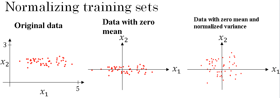
The input features x are two dimensional i.e. \( x_1, x_2 \), and the scatter plot of your training set is shown above.

Normalizing your inputs corresponds to two steps.

The first is to subtract out or to zero out the mean. This is done by setting \( \mu = \frac{1}{m} \sum_{i = 1}^{m} x_i \).

\( \mu \) is a vector of means, and then we subtract the mean from every training example, so in effect you just move the training set until it has zero mean.

And then the second step is to normalize the variances. So notice here that the feature \( x_1 \) has a much larger variance than the feature \( x_2 \).

So what we do is set \( (\sigma)^2 = \frac{1}{m} \sum_{i = 1}^{m} (x_i)^2 \). And so now sigma squared is a vector with the variances of each of the features

And you take each example and divide it by this vector sigma squared. And so in pictures, you end up with the third image. Where now the variance of \( x_1 \) and \( x_2 \) are both equal to one.

And one tip, if you use this to scale your training data, then use the same \( \mu \) and \( \sigma^2 \) to normalize your test set

In particular, you don't want to normalize the training set and the test set differently.

Because you want your data, both training and test examples, to go through the same transformation defined by the same \( \mu \) and \( \sigma^2 \) calculated on your training data.

Recall that a cost function is defined as : \( J(w, b) = \frac{1}{m} \sum_{i=1}^{m} L(\hat{y}^{(i)} , y^{(i)})\)

If you use unnormalized input features, it's more likely that your cost function will look like a very squished out bowl, very elongated cost function, where the minimum you're trying to find is difficult to reach.

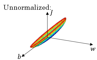
But if your features are on very different scales, say the feature X1 ranges from 1 to 1,000, and the feature X2 ranges from 0 to 1, then it turns out that the ratio or the range of values for the parameters w1 and w2 will end up taking on very different values.

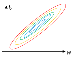
And so maybe these axes should be w1 and w2, but I'll plot w and b, then your cost function can be a very elongated bowl like the one given above.

So if you part the contours of this function, you can have a very elongated function like that.

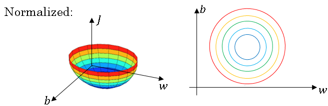
Whereas if you normalize the features, then your cost function will on average look more symmetric.

And if you're running gradient descent on the cost function on the unnormalized training data, then you might have to use a very small learning rate because gradient descent might need a lot of steps to oscillate back and forth before it finally finds its way to the minimum.

Whereas if you have a more spherical contours, then wherever you start gradient descent can pretty much go straight to the minimum.

You can take much larger steps with gradient descent rather than needing to oscillate around.

Of course in practice w is a high-dimensional vector, and so trying to plot this in 2D doesn't convey all the intuitions correctly. But the rough intuition that your cost function will be more round and easier to optimize when your features are all on similar scales (-1 to 1).

That just makes your cost function J easier and faster to optimize.

In practice if one feature, say X1, ranges from zero to one, and X2 ranges from minus one to one, and X3 ranges from one to two, these are fairly similar ranges, so this will work just fine.

It's when they're on dramatically different ranges like ones from 1 to a 1000, and the another from 0 to 1, that that really hurts your optimization algorithm.

But by just setting all of them to a 0 mean and say, variance 1, like we did using the previous formula, that just guarantees that all your features on a similar scale and will usually help your learning algorithm run faster.

So, if your input features came from very different scales, maybe some features are from 0 to 1, some from 1 to 1,000, then it's important to normalize your features.

If your features came in on similar scales, then this step is less important.

Although performing this type of normalization never does any harm, so we often do it anyway if we are not sure whether or not it will help with speeding up training for your algebra.