Exploratory Data Analysis and Statistics
Statistics is therefore a process in which
Collect data
Summarize data
Interpret data
The process of statistics starts when we identify what group we want to study or learn something about. We call this group the population.
Population, then, is the entire group that is the target of our interest. In most cases, the population is so large that, as much as we want to, there is absolutely no way we can study all of it. A more practical approach would be to examine and collect data only from a subgroup of the population, which we call a sample. We call this first step, which involves choosing a sample and collecting data from it, producing data.
Since, for practical reasons, we need to compromise and examine only a sub-group of the population rather than the whole population, we should make an effort to choose a sample in such a way that it will represent the population well.
Once the data have been collected we need to summarize that list in a meaningful way. This second step, which consists of summarizing the collected data, is called exploratory data analysis.
We want is to be able to draw conclusions about the population based on the sample results. Before we can do so, we need to look at how the sample we're using may differ from the population as a whole, so that we can factor that into our analysis. To examine this difference, we use probability.
Finally, we can use what we've discovered about our sample to draw conclusions about our population. We call this final step in the process inference.
Four Steps of Statistics
Producing Data : Choosing a sample from the population of interest and collecting data.
Exploratory Data Analysis (EDA) Summarizing the data we've collected.
Probability and Inference: Drawing conclusions about the entire population based on the data collected from the sample.
Data and Variables
Data are pieces of information about individuals organized into variables. By an individual, we mean a particular person or object. By a variable, we mean a particular characteristic of the individual.
A dataset is a set of data identified with particular circumstances. Datasets are typically displayed in tables, in which rows represent individuals and columns represent variables.
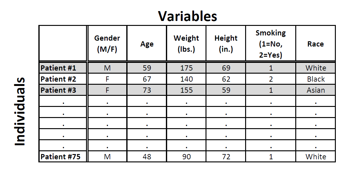
Example: Medical Records
In this example, the individuals are patients, and the variables are Gender, Age, Weight, Height, Smoking, and Race. Each row, then, gives us all the information about a particular individual (in this case, patient), and each column gives us information about a particular characteristic of all the patients
Variables can be classified into one of two types: categorical or quantitative
Categorical variables take category or label values and place an individual into one of several groups. Each observation can be placed in only one category, and the categories are mutually exclusive. In our example of medical records, Smoking is a categorical variable, with two groups, since each participant can be categorized only as either a nonsmoker or a smoker. Gender and Race are the two other categorical variables in our medical records example. They have no arithmetic meaning (i.e., it does not make sense to add, subtract, multiply, divide, or compare the magnitude of such values). E.g: GPS location, Pin code
Quantitative variables take numerical values and represent some kind of measurement. In our medical example, Age is an example of a quantitative variable because it can take on multiple numerical values. Weight and Height are also examples of quantitative variables.
Categorical variables are sometimes called qualitative variables
Scales of Measurement / Types of Variable
There is a more precise method of categorizing variables: it is called scale of measurement. The scales of measurement become increasingly precise with each level while retaining the characteristics of the level below it. The four different scales of measurement, from least to most precise, are given as:
Nominal : It is the least precise measure of data as it only indicates differences. Nominal level data uses discrete categories to describe qualitative differences. An example of a nominal variable is types of pets. For instance, types of pets can include birds, fish, cats, and dogs. None of these categories – in this case types of pets – is implicitly better than the other. Rather, the categories reflect the different types of pets. Some other examples of nominal variables include gender, eye color, type of house, and type of resident. The categories for each of these nominal variables reflect qualitative differences but quantitative. Quantitative differences are less than, greater than etc.
Ordinal : Ordinal level data is more precise than nominal data as the differences can now be rank ordered. However, it does not indicate that the differences between two numbers are fixed or equal An example of an ordinal variable is the order of finishes in a race. For instance, we can say that John finished first and Alex finished second. However, we do not know the degree of difference. It could be that John won by 2 seconds or 20 minutes. Other examples of ordinal variables include education level. The categories for each of these ordinal variables show order, but not the magnitude of difference between two adjacent points.
Interval : It builds upon the characteristics of ordinal data through the addition of meaningful differences between two numbers – that is, the distance between pairs of consecutive numbers is assumed to be equal. However, interval variables do not have a meaningful zero point. Thus, a zero does not mean the absence of an attribute, but rather, is a particular, but arbitrary, point on the scale. For instance, when temperature is measured in Celsius, the one degree difference, say, between 35 degrees and 36 degrees is assumed to be the same as one degree difference between 25 degrees and 26 degrees. However, zero degrees in Celsius does not mean the absence of heat since there are below freezing temperatures such as twenty below. The same characteristics also hold true for temperatures measured in Fahrenheit. Some other examples of interval variables include IQ scores and SAT scores. For each of these interval variables, the distance between pairs of consecutive numbers is assumed to be equal, but they do not have a meaningful zero point.
Ratio : It has all the characteristics of interval data plus a meaningful zero point. A good example of ratio level data is age. For instance, we know that someone who is forty years old is twice as old as someone who is twenty years old. There is a meaningful zero point – that is, it is possible to have the absence of age. Some other examples of ratio variables include height, weight, cost of a car in dollars. For each of these ratio variables the distance between pairs of consecutive numbers as assumed to be equal and there is a meaningful zero point.
It is also important to note that more precise data can always be scaled down to less precise data. For instance, a ratio level variable like age can be scaled into an ordinal variable of age groups, which could include toddler, adolescent, young adult, and middle aged
Less precise data, however, cannot be made into more precise data – that is, an ordinal level variable like age groups cannot be changed into a ratio level variable such as age in years.
Statistical methods are ways of summarizing, analyzing, and interpreting data, and are designed for specific types of data. Researchers need to know the level of measurement of their data when selecting a statistical method since using an incorrect method for analyzing data can affect the reliability and accuracy of the results. Be sure to keep these levels of measurement in mind whenever you are planning to analyze data.