Researchers discovered at the beginning of the 20th century that human blood comes in various types (A, B, AB, and O), and that some types are more common than others.

How could researchers determine the probability of a particular blood type, say O? Just looking at one or two or a handful of people would not be very helpful in determining the overall chance that a randomly chosen person would have blood type O.

But sampling many people at random, and finding the relative frequency of blood type O occurring, provides an adequate estimate. For example, it is now well known that the probability of blood type O among white people in the United States is 0.45.

This was found by sampling many (say, 100,000) white people in the country, finding that roughly 45,000 of them had blood type O, and then using the relative frequency: 45,000 / 100,000 = 0.45 as the estimate for the probability for the event "having blood type O."

(Comment: Note that there are racial and ethnic differences in the probabilities of blood types. For example, the probability of blood type O among black people in the United States is 0.49, and the probability that a randomly chosen Japanese person has blood type O is only 0.3).

To estimate the probability of event A, written P(A), we may repeat the random experiment many times and count the number of times event A occurs. Then P(A) is estimated by the ratio of the number of times A occurs to the number of repetitions, which is called the relative frequency of event A.

Relative frequency of event A = \( \frac{\text{number of times A occurs}}{\text{total number of repetitions}} \)

The Law of Large Numbers states that as the number of trials increases, the relative frequency becomes the actual probability. So, using this law, as the number of trials increases, the empirical probability gets closer and closer to the theoretical probability.

Principle Law of Large Numbers: The actual (or true) probability of an event (A) is estimated by the relative frequency with which the event occurs in a long series of trials.

Comments:

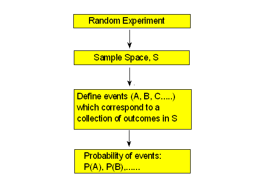
Probability questions arise when we are faced with a situation that involves uncertainty. Such a situation is called a random experiment, an experiment that produces an outcome that cannot be predicted in advance (hence the uncertainty).

Here are a few examples of random experiments:

Comment: Does Order Matter? Note that when a coin is tossed twice, as in example 2, the possible outcome HT (indicating that the first toss was H and the second T) is NOT the same as the outcome TH (indicating that T occurred first and then H), and therefore both outcomes were listed separately. This is an example of a situation when order does matter. However, order does not always matter. Example 6 is a case in which order does not matter. The outcome (Ann, Beth) indicates that Ann and Beth are the two randomly chosen to get the jobs. Whether Ann appears first or Beth does is irrelevant in this case, and therefore (Beth, Ann) was not listed as a separate outcome.

There is really no rule that dictates when order matters and when it doesn't. It is sometimes clear from the way the random experiment is defined. For example, suppose I were to change example 6 slightly:

There are two job openings for similar staff positions at a certain college: one in the Registrar's Office, and one in the Office of Admissions. The Human Resources Department has identified four equally qualified candidates for the jobs (Ann, Beth, Jim and Dan), and for fairness decides to choose two of the four candidates at random. The first chosen will fill the position in the Registrar's Office, and the second will fill the position in the Office of Admissions.

Now order is relevant—the two outcomes (Ann, Beth) and (Beth, Ann) are not the same in this scenario. The first outcome indicates that Ann got the position at the Registrar's Office and Beth got the position at the Office of Admissions, while the second outcome indicates the reverse. In this case, therefore, all the possible outcomes are:

{ (Ann, Beth), (Beth, Ann), (Ann, Jim), (Jim, Ann), (Ann, Dan), (Dan, Ann),

(Beth, Jim), (Jim, Beth), (Beth, Dan), (Dan, Beth), (Jim, Dan), (Dan, Jim) }

Each random experiment has a set of possible outcomes, and there is uncertainty as to which of the outcomes we are actually going to get once the experiment is conducted. This list of possible outcomes is called the sample space of the random experiment, and is denoted by the (capital) letter S.

Going back to the 6 examples above, we can write:

Once we have defined a random experiment, we can talk about an event of interest, which is a statement about the nature of the outcome that we're actually going to get once the experiment is conducted. Events are denoted by capital letters (other than S, which is reserved for the sample space).

Example: Tossing a Coin 3 Times Consider example 3, tossing a coin three times. Recall that the sample space in this case is:

S = {HHH, THH, HTH, HHT, HTT, THT, TTH, TTT}

We can define the following events:

Note that each event is indeed a statement about the outcome that the experiment is going to produce.

In practice, each event corresponds to some collection (subset) of the outcomes in the sample space:

Here is a visual representation of events A, B and C.

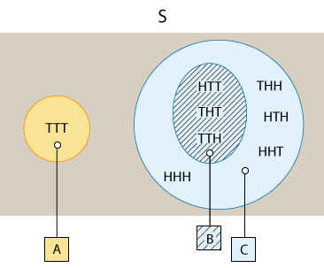
From this visual representation of the events, it is easy to see that event B is totally included in event C, in the sense that every outcome in event B is also an outcome in event C. Also, note that event A stands apart from events B and C, in the sense that they have no outcome in common, or no overlap. At this point these are only noteworthy observations.

Example: Staff Position Consider Example 6, where we choose two candidates at random out of four (Ann, Beth, Jim and Dan). Recall that in this case the sample space is:

S = { (Ann, Beth), (Ann, Jim), (Ann, Dan), (Beth, Jim), (Beth, Dan), (Jim, Dan) }

In this example, we might be interested in the following events, each of which is a statement about the nature of the outcome that the random experiment will produce:

Event A: "Jim is chosen."

Event B: "The two chosen are of the same gender."

Again, each event corresponds to some collection of outcomes. Use the exercise below to try this yourself:

Once an event is defined, we can talk about the probability that it will occur. So, if we have defined an Event A, we can use the notation we previously mentioned to represent its probability, namely P(A).

The following figure summarizes the information in this section:

In the previous section we considered situations in which all the possible outcomes of a random experiment are equally likely, and learned a simple way to find the probability of any event in this special case.

We are now moving on to learn how to find the probability of events in the general case (when the possible outcomes are not necessarily equally likely), using five basic probability rules.

Fortunately, these basic rules of probability are very intuitive, and as long as they are applied systematically, they will let us solve more complicated problems; in particular, those problems for which our intuition might be inadequate.

Rule 1 : For any event A, 0 ≤ P(A) ≤ 1.

This first rule simply reminds us of the basic property of probability that we've already learned. The probability of an event, which informs us of the likelihood of it occurring, can range anywhere from 0 (indicating that the event will never occur) to 1 (indicating that the event is certain).

One practical use of this rule is that is can be used to identify any probability calculation that comes out to be more than 1 as wrong.

Before moving on to the other rules, let's first look at an example that will provide a context for illustrating the next several rules.

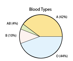
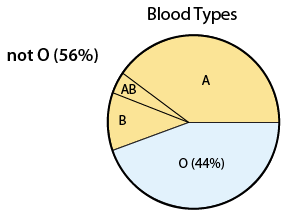
Example : As previously discussed, all human blood can be typed as O, A, B or AB. In addition, the frequency of the occurrence of these blood types varies by ethnic and racial groups.

According to Stanford University's Blood Center , these are the probabilities of human blood types in the United States (the probability for type A has been omitted on purpose):

Motivating question for rule 2: A person in the United States is chosen at random. What is the probability of the person having blood type A?

Answer : Our intuition tells us that since the four blood types O, A, B, and AB exhaust all the possibilities, their probabilities together must sum to 1, which is the probability of a "certain" event (a person has one of these 4 blood types for certain). Since the probabilities of O, B, and AB together sum to 0.44 + 0.1 + 0.04 = 0.58, the probability of type A must be the remaining 0.42 (1 - 0.58 = 0.42):

This example illustrates our second rule, which tells us that the probability of all outcomes in the sample space together must be 1.

Rule 2 : P(S) = 1; that is, the sum of the probabilities of all possible outcomes is 1.

Comment This is a good place to compare and contrast what we're doing here with what we learned in the Exploratory Data Analysis (EDA) section. Notice that in this problem we are essentially focusing on a single categorical variable: blood type. We summarized this variable above, as we summarized single categorical variables in the EDA section, by listing what values the variable takes and how often it takes them. In EDA we used percentages, and here we're using probabilities, but the two convey the same information. In the EDA section, we learned that a pie chart provides an appropriate display when a single categorical variable is involved, and similarly we can use it here (using percentages instead of probabilities):

Even though what we're doing here is indeed similar to what we've done in the EDA section, there is a subtle but important difference between the underlying situations in this section and the ones in the Exploratory Data Analysis section.

In EDA, we summarized data that were obtained from a sample of individuals for whom values of the variable of interest were recorded. Here, when we present the frequency, or probability, of each blood type, we have in mind the entire population of people in the United States, for which we are presuming to know the overall frequency of values taken by the variable of interest.

Marital status can be categorized into: never married, married, widowed or divorced. According to Infoplease.com, the following are the probabilities of those marital status categories for adults in the United States (data from 2000):

In probability and in its applications, we are frequently interested in finding out the probability that a certain event will not occur.

An important point to understand here is that "event A does not occur" is a separate event that consists of all the outcomes in the sample space S that are not in A.

It is for this reason that the event "event A does not occur" is called "the complement event of A," since it compares event A to the whole sample space. Notation: we will write "not A" to denote the event that A does not occur.

Here is a visual representation of how event A and its complement event "not A" together represent the whole sample space.

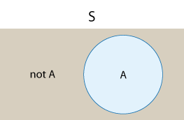
Comment Such a visual display is called a "Venn diagram." A Venn diagram is a simple way to visualize events and the relationships between them using rectangles and circles. We will use Venn diagrams throughout this module.

Rule 3 deals with the relationship between the probability of an event and the probability of its complement event. Given that event A and event "not A" together make up the whole sample space S, and since rule 2 tells us that P(S) = 1, the following rule should be quite intuitive:

Rule 3: The Complement Rule P(not A) = 1 - P(A); that is, the probability that an event does not occur is 1 minus the probability that it does occur.

Example Back to the blood type example:

Here is some additional information:

Comment Note that the Complement Rule, P(not A) = 1 - P(A) can be re-formulated as P(A) = 1 - P(not A). This seemingly trivial algebraic manipulation has an important application, and actually captures the strength of the complement rule. In some cases, when finding P(A) directly is very complicated, it might be much easier to find P(not A) and then just subtract it from 1 to get the desired P(A). We will come back to this comment and see examples later in this module.

On the "Information for the Patient" label of a certain antidepressant it is claimed that based on some clinical trials, when taking this medication

- there is a 14% chance of experiencing sleeping problems, or insomnia (denote this event by I)

- there is a 26% chance of experiencing headaches (denote this event by H), and

- there is a 35% chance of experiencing at least one of these two side effects (denote this event by L)

Finding P(A or B), the probability of one event or another occurring. Before we get to the actual rule, however, we need some clarifications and definitions.

When a parent says to his or her child in a toy store "Do you want toy A or toy B?", this means that the child is going to get only one toy and he or she has to choose between them. Getting both toys is usually not an option.

In contrast, In probability, "OR" means either one or the other or both. and so, P(A or B) = P(event A occurs or event B occurs or both occur)

Having said that, it should be noted that there are some cases where it is simply impossible for the two events to both occur at the same time, in which case we don't have to worry about the possibility that both occur when we try to find P(A or B). The distinction between events that can happen together and those that cannot is an important one.

Example Consider the following two events: A—a randomly chosen person has blood type A, and B—a randomly chosen person has blood type B.

In rare cases, it is possible for a person to have more than one type of blood flowing through his or her veins, but for our purposes, we are going to assume that each person can have only one blood type. Therefore, it is impossible for the events A and B to occur together.

Example Consider the following two events: A—a randomly chosen person has blood type A B—a randomly chosen person is a woman.

In this case, it is possible for events A and B to occur together.

Definition: Two events that cannot occur at the same time are called disjoint or mutually exclusive. (We will use disjoint.)

We can therefore say that in the first example events A and B are disjoint, and in the second example they are not disjoint. Using Venn diagrams, we can visualize two events that are disjoint and compare them to two events that are not:

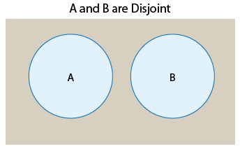
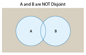
The Venn diagrams suggest that another way to think about disjoint versus not disjoint events is that disjoint events do not overlap. They do not share any of the possible outcomes, and therefore cannot happen together. On the other hand, events that are not disjoint are overlapping in the sense that they share some of the possible outcomes and therefore can occur at the same time.

A couple that is planning to have 3 children, where the sample space S of all possible outcomes is: S={BBB, BBG, BGB, GBB, GGB, GBG, BGG, GGG} Consider the following two events:

i. Here are the possible outcomes in each of the events:

A={BGB, GGB, BGG, GGG}

iii. Based on ii, the events are not disjoint since, they can happen together, if the couple ends up having three girls.

Consider the following two events:
A—exactly one of the three children is a girl
C—exactly one of the three children is a boy.

i. What are the possible outcomes for each of these events?
ii. Do the events share any of the outcomes? (i.e., is there an overlap between the two events?)
iii. Based on ii, are the events disjoint or not?

i. Here are the possible outcomes in each of the events:
A={GBB, BGB, BBG}
C={BGG, GBG, GGB}
ii. The events do not overlap; they have no outcome in common.
iii. Based on ii, the events are disjoint—they can never occur together.

A couple decides to have children until they have one boy and one girl, but they will not have more than three children. The sample space of possible outcomes is S = {GB, BG, BBG, GGB, BBB, GGG}.
Consider the following events:
A–the couple has one boy
C–the couple has three children
D–all of the children are the same gender