• Just like any other variable, random variables can take on multiple values. What differentiates random variables from other variables is that the values for these variables are determined by a random trial, random sample, or simulation.




• The probabilities for the values can be determined by theoretical or observational means. Such probabilities play a vital role in the theory behind statistical inference, our ultimate goal in this course.




• Random variable (definition) A random variable assigns a unique numerical value to the outcome of a random experiment. A random variable can be thought of as a function that associates exactly one of the possible numerical outcomes to each trial of a random experiment. However, that number can be the same for many of the trials.




• Example: Theoretical Consider the random experiment of flipping a coin twice. The sample space of possible outcomes is S = { HH, HT, TH, TT }.




• Now, let's define the variable X to be the number of tails that the random experiment will produce.




1. If the outcome is HH, we have no tails, so the value for X is 0.




2. If the outcome is HT, we got one tail, so the value for X is 1.




3. If the outcome is TH, we again got one tail, so the value for X is 1.




4. Lastly, if the outcome is TT, we got two tails, so the value for X is 2.




• As the definition suggests, X is a quantitative variable that takes the possible values of 0, 1, or 2.




• It is random because we do not know which of the three values the variable will eventually take. We can ask questions like:




• As you can see, random variables are not really a new thing, but just a different way to look at the same problem.




• Note that if we had tossed a coin three times, the possible values for the number of tails would be 0, 1, 2, or 3. In general, if we toss a coin "n" times, the possible number of tails would be 0, 1, 2, 3, ... , or n.




• Example: Observational Consider getting data from a random sample on the number of ears in which a person wears one or more earrings.




• We define the variable X to be the number of ears in which a randomly selected person wears an earring.




1. If the selected person does not wear any earrings, then X = 0.




2. If the selected person wears earrings in either the left or the right ear, then X = 1.




3. If the selected person wears earrings in both ears, then X = 2.




• As the definition suggests, X is a quantitative variable which takes the possible values of 0, 1, or 2. We can ask questions like:




1. What is the probability that a randomly selected person will have earrings in both ears?




2. What is the probability that a randomly selected person will not be wearing any earrings in either ear?




• NOTE... We identified the first example as theoretical and the second as observational. Let's discuss the distinction.




• To answer probability questions about a theoretical situation, we only need the principles of probability. However, if we have an observational situation, the only way to answer probability questions is to use the relative frequency we obtain from a random sample.




• Here is a different type of example:




• Example: Lightweight Boxer Assume we choose a lightweight male boxer at random and record his exact weight. According to the boxing rules, a lightweight male boxer must weigh between 130 and 135 pounds, so the sample space here is S = { All the numbers in the interval 130-135 }. (Note that we can't list all the possible outcomes here.)




• We'll define X to be the weight of the boxer (again, as the definition suggests, X is a quantitative variable whose value is the result of our random experiment). Here X can take any value between 130 and 135. We can ask questions like:




1. What is the probability that X will be more than 132? In other words, what is the probability that the boxer will weigh more than 132 pounds?




2. What is the probability that X will be between 131 and 133? In other words, what is the probability that the boxer weighs between 131 and 133 pounds?




3. What is the difference between the random variables in these examples? Let's see:




• They all arise from a random experiment (tossing a coin twice, choosing a person at random, choosing a lightweight boxer at random).




• They are all quantitative (number of tails, number of ears, weight).




• Where they differ is in the type of possible values they can take: In the first two examples, X has three distinct possible values: 0, 1, and 2. You can list them. In contrast, in the third example, X takes any value in the interval 130-135, and thus the possible values of X cover an infinite range of possibilities, and cannot be listed.




• A random variable like the one in the first two examples, whose possible values are a list of distinct values, is called a discrete random variable. A random variable like the one in the third example, that can take any value in an interval, is called a continuous random variable.




• Just as the distinction between categorical and quantitative variables was important in Exploratory Data Analysis, the distinction between discrete and continuous random variables is important here, as each one gets a different treatment when it comes to calculating probabilities and other quantities of interest.

• Comments Sometimes, continuous random variables are "rounded" and are therefore "in a discrete disguise."




• For example :




1. time spent watching TV in a week, rounded to the nearest hour (or minute)




2. outside temperature, to the nearest degree




3. a person's weight, to the nearest pound.




• Even though they "look like" discrete variables, these are still continuous random variables, and we will in most cases treat them as such.




• On the other hand, there are some variables which are discrete in nature, but take so many distinct possible values that it will be much easier to treat them as continuous rather than discrete.




1. the IQ of a randomly chosen person




2. the SAT score of a randomly chosen student




3. the annual salary of a randomly chosen CEO, whether rounded to the nearest dollar or the nearest cent




• Sometimes we have a discrete random variable but do not know the extent of its possible values. For example: How many accidents will occur in a particular intersection this month? We may know from previously collected data that this number is from 0-5. But, 6, 7, or more accidents could be possible.




• A good rule of thumb is that discrete random variables are things we count, while continuous random variables are things we measure.




• We counted the number of tails and the number of ears with earrings. These were discrete random variables.




• We measured the weight of the lightweight boxer. This was a continuous random variable.




• Often we can have a subject matter for which we can collect data that could involve a discrete or a continuous random variable, depending on the information we wish to know.




• Example: Soft Drinks Suppose we want to know how many days per week you drink a soft drink. The sample space would be S = { 0, 1, 2, 3, 4, 5, 6, 7 }. There are a finite number of values for this variable. This would be a discrete random variable.




• Instead, suppose we want to know how many ounces of soft drinks you consume per week. Even if we round to the nearest ounce, the answer is a measurement. Thus, this would be a continuous random variable.




• Example: x-bar Suppose we are interested in the weights of all males. We take a random sample and get the mean for that sample, namely \( \overline{x} \). We then take another random sample (with the same sample size) and get another \( \overline{x} \).




• We would expect the values of the \( \overline{x} \)s from these two samples to be different, but pretty close in value.




• Each time we take a sample we'll get a different \( \overline{x} \). We will take lots of samples and thus get many \( \overline{x} \)s.




• The value of \( \overline{x} \) from these repeated samples is a random variable. Since it can take on any value within an interval of possible male weights it is a continuous random variable.


A fair coin is tossed twice. Let the random variable X be the number of tails we get in this random experiment. In this case, the possible values that X can assume are 0 (if we get HH), 1 (if get HT or TH) , and 2 (if we get TT).



• Notation




1. If we want to find the probability of the event "getting 1 tail," we'll write: P(X = 1)




2. If we want to find the probability of the event "getting 0 tails," we'll write: P(X = 0)




3. In general, we'll write: P(X = x) to denote the probability that the discrete random variable X gets the value x.




4. Note that for the random variables we'll use a capital letter, and for the value we'll use a lowercase letter.

View Answer



View Answer



View Answer



View Answer



View Answer



View Answer

• All the possible values of a discrete random variable, along with their associated probabilities can be displayed as a list. This list of possible values and probabilities is called the probability distribution of the random variable




• Example: Flipping a Coin Twice What is the probability distribution of X, where the random variable X is the number of tails appearing in two tosses of a fair coin?




• We first note that since the coin is fair, each of the four outcomes HH, HT, TH, TT in the sample space S is equally likely, and so each has a probability of 1/4. (Alternatively, the multiplication principle can be applied to find the probability of each outcome to be 1/2 * 1/2 = 1/4.)




• 




1. X takes the value 0 only for the outcome HH, so the probability that X = 0 is 1/4.




2. X takes the value 1 for outcomes HT or TH. By the addition principle, the probability that X = 1 is 1/4 + 1/4 = 1/2.




3. Finally, X takes the value 2 only for the outcome TT, so the probability that X = 2 is 1/4.




• 




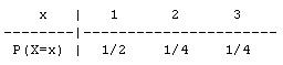
• The probability distribution of the random variable X is easily summarized in a table:




• 




• As mentioned before, we write "P(X = x)" to denote "the probability that the random variable X takes the value x."




• The way to interpret this table is:




1. X takes the values 0, 1, 2 and P(X = 0) = 1/4, P(X = 1) = 1/2, P(X = 2) = 1/4.




• Note that events of the type (X = x) are subject to the principles of probability established earlier, and will provide us with a way of systematically exploring the behavior of random variables. In particular, the first two principles in the context of probability distributions of random variables will now be stated.




• Any probability distribution of a discrete random variable must satisfy:




1. \( 0 \leq P(X=x) \leq 1 \)




2. \( \sum_x P(X=x) = 1 \)

• A coin is tossed three times. Let the random variable X be the number of tails. Find the probability distribution of X.




• First, we specify the 8 possible outcomes in S, along with the number and the probability of that outcome. (Because they are all equally likely, each has probability 1/8. Alternatively, by the multiplication principle, each particular sequence of three coin faces has probability 1/2 * 1/2 * 1/2 = 1/8.)




• 




• Next, we figure out what the value of X is (number of tails) for each possible outcome.




• 




• Next, we use the addition principle to assert that




• P(X = 1) = P(HHT or HTH or THH) = P(HHT) + P(HTH) + P(THH) = 1/8 + 1/8 + 1/8 = 3/8.




• Similarly, P(X = 2) = P(HTT or THT or TTH) = 3/8.




• 




• The resulting probability distribution is:




• 

• A young couple decides to try to have children until they have a boy. For financial reasons, the couple decides that they are going to stop trying when they have three children, whether they have a boy or not. (We are assuming that having a boy or a girl is equally likely, and that the child's gender in each birth is independent of the gender in the other births.)




• Let the random variable X be the number of children the couple has.




• Our goal is to find the probability distribution of X. In other words, we would like to create a table that lists all the possible values of X and the corresponding probabilities. We'll follow the same steps we followed in the two examples we solved.




• What is the sample space S in this case? In other words, what are all the possible outcomes in this case? (Use B for a boy and G for a girl).




1. There are four possible outcomes in this case:




2. B—the first child is a boy, and the couple stops having children.




3. GB—the first child is a girl and the second is a boy, and then the couple stops having children.




4. GGB—the first and second child are girls and the third is a boy, and the couple stops having children.




5. GGG—all three children are girls but the couple stops having children for financial reasons.




• Using simple principles of probability, find the probability of each of the outcomes listed in the previous question.




1. P(B) = 1/2




2. P(GB) = 1/2 * 1/2 = 1/4 (using the multiplication principle for independent events)




3. P(GGB) = 1/2 * 1/2 * 1/2 = 1/8 (using the multiplication principle for independent events)




4. P(GGG) = 1/2 * 1/2 * 1/2 = 1/8 (using the multiplication principle for independent events)




• Write down the value of the random variable X that is associated with each outcome.




1. For B, X = 1 (the couple has just one child)




2. For GB, X = 2 (the couple has two children)




3. For GGB, X = 3 (the couple has three children)




4. For GGG, X = 3 (the couple has three children)




• Using what you found in the question above, summarize the probability distribution of X in a table.




1. 




2. Note that P(X = 3) = 1/4 since by the addition principle (for disjoint events):




3. P(X = 3) = P(GGB) + P(GGG) = 1/8 + 1/8 = 1/4

• Example: Formulas to Define Random Variable




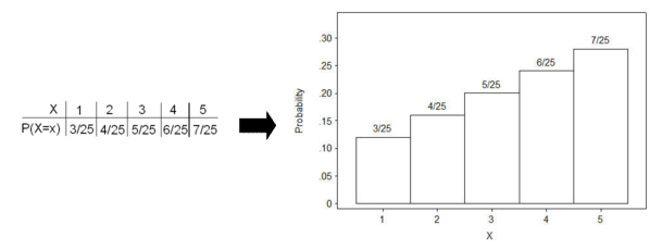
• A random variable X has a probability distribution of P(X = x) = (x + 2) / 25 for x = 1, 2, 3, 4, 5.




• Show the probability distribution in a table, and verify that the above requirements are satisfied. Substituting x = 1, 2, 3, 4, and 5, respectively, into the formula for P(X = x), we have




• Clearly, each probability is between 0 and 1. Also, the probabilities sum to (3 + 4 + 5 + 6 + 7) / 25 = 25/25 = 1.




• Scenario: Telemarking Sales The number of sales that a telemarketing salesperson makes in an hour is a random variable X having the following probability distribution: P(X = x) = (x + 2)(5-x) / 50 for x = 0, 1, 2, 3, 4




• Which of the following tables represents the probability distribution of X?




• Table D - This is the right probability distribution. In order to find the probability that X takes a certain value, you need to plug that value into the formula. So, for example, P(X = 1) = (1 + 2)(5 - 1) / 50 = 12/50. Note that this is a legitimate probability distribution since all the probabilities are between 0 and 1, and their sum is 1.

• We learned to display the distribution of sample values for a quantitative variable with a histogram in which the horizontal axis represented the range of values in the sample. The vertical axis represented the frequency or relative frequency (sometimes given as a percentage) of sample values occurring in that interval. So the width of each rectangle in the histogram was an interval, or part of the possible values for the quantitative variable, and the height of each rectangle was the frequency (or relative frequency) for that interval.




• Similarly, we can display the probability distribution of a random variable with a probability histogram. The horizontal axis represents the range of all possible values of the random variable, and the vertical axis represents the probabilities of those values.




• Here is the probability histogram for the previous example:




• A two row probability distribution table, in which the rows are labeled "X" and "P(X=x)." Data is given in column oriented format (X: P(X=x)): 1: 3/25; 2: 4/25; 3: 5/25; 4: 6/25; 5: 7/25; along with The histogram generated from the table. The vertical axis is labeled "Probability" and the horizontal axis is labeled "X.". The histogram contains vertical bars at which are centered on the value x for which they represent on the horizontal axis, and the bars are as tall as the probability P(X = x).




• 




• Area of a Probability Histogram




• Notice that each rectangle in the histogram has a width of 1 unit. The height of each rectangle is the probability that it will occur. Thus, the area of each rectangle is base times height, which for these rectangles is 1 times its probability for each value of X. This means that the sum of the areas of all of the rectangles is the same as the sum of all of the probabilities. Therefore, the total area = 1.




• Using the completed probability distribution below, explain why it is indeed a legitimate probability distribution.




• 




• To be a probability distribution, two conditions must be satisfied.




• 1. Each of the probabilities must be between 0 and 1. Certainly 0.28, 0.34, 0.18, 0.14, and 0.06 are all between 0 and 1.




• 2. The sum of all of the probabilities must equal 1. Indeed, 0.28 + 0.34 + 0.18 + 0.14 + 0.06 = 1.




• Using the completed probability distribution below, show that the sum of the areas of all of the rectangles is one.




• 




• The sum of the areas = 1(.28) + 1(.34) + 1(.18) + 1(.14) + 1(.06) = 1.




• This make sense, since 1(.28) + 1(.34) + 1(.18) + 1(.14) + 1(.06) = 0.28 + 0.34 + 0.18 + 0.14 + 0.06, which we already know is equal to 1.

• Based upon data collected in the 2000 United States Census and an expanded number of households, the following histogram was constructed. It shows the distribution of people per household.




• 

View Answer

• The probability distribution of the random variable X is represented by the following histogram.




• Fill in the probability distribution table values consistent with the histogram above:




• Cell 1 : 0.4 Cell 2 : 2




• Cell 3 : 3 Cell 4 : 0.1




• The probability distribution represented in the histogram and table above may be also expressed by which formula? P(X = x) = (5 - x) / 10 for x = 1, 2, 3, 4 Using this formula, we'll get P(X = 1) = (5 - 1) / 10 = 0.4, P(X = 2) = (5 - 2) / 10 = 0.3, P(X = 3) = (5 - 3) / 10 = 0.2, P(X = 4) = (5 - 4) / 10 = 0.1, which is exactly the one represented by the histogram above

• Example: Changing Majors A random sample of graduating seniors was surveyed just before graduation. One question that was asked is: How many times did you change majors? The results are displayed in a probability distribution.




• 




• Using this probability distribution we can answer probability questions such as: What is the probability that a randomly selected senior has changed majors more than once? This can be written as P(X > 1).




• More than once would be translated to:




1. P(X > 1) = P(X = 2) + P(X = 3) + P(X = 4) + P(X = 5)




2. P(X > 1) = 0.23 + 0.09 + 0.02 + 0.01




3. P(X > 1) = 0.35




• As you just saw in this example, we need to pay attention to the wording of the probability question. The key words that told us which values to use for X are more than. The following will clarify and reinforce the key words and their meanings.




• The following table gives a list of some key words to know. Suppose a random variable X had possible values of 0-5.




• Key Words	Meaning	Symbols	Values for X
  more than 2	strictly larger than 2	X > 2	3, 4, 5
  no more than 2	2 or fewer	X ≤ 2	0, 1, 2
  fewer than 2	strictly smaller than 2	X < 2	0, 1
  no less than 2	2 or more	X ≥ 2	2, 3, 4, 5
  at least 2	2 or more	X ≥ 2	2, 3, 4, 5
  at most 2	2 or fewer	X ≤ 2	0, 1, 2
  exactly 2	2, no more or no less, only 2	X = 2	2




• Before we move on to the next section on the means and variances of a probability distribution, let's revisit the changing majors example:




• 




• Question: Based upon this distribution, do you think it would be unusual to change majors 2 or more times?




• Answer: P(X ≥ 2) = 0.35. So, 35% of the time a student changes majors 2 or more times. This means that it is not unusual to do so.




• Question: Do you think it would be unusual to change majors 4 or more times?




• Answer: P(X ≥ 4) = 0.03. So, 3% of the time a student changes majors 4 or more times. This means that it is fairly unusual to do so.

View Answer



View Answer



View Answer

• An article reviews the overwhelming scientific evidence that establishes that eyewitnesses are notoriously inaccurate in identifying strangers, especially under the conditions that exist in many serious offenses such as robbery. Many of the factors that tend to decrease the accuracy of an identification are intrinsic to a witness’ abilities, and not the product of inappropriate suggestion by the police.




• We know, for example, that eyewitnesses identify a known wrong person (a “filler” or “foil”) in approximately 20% of all real criminal lineups.




• Using the data that 20% of eyewitnesses identify a known wrong person, we wish to create a probability distribution and answer some probability questions.




• Suppose we have three randomly selected lineups. Let I represent an incorrect identification.




• Note: The complement of I is that an incorrect identification has not occurred. This means that in any randomly selected lineup either the correct person or nobody was identified. In either case nothing incorrect has happened. So, for simplicity, let C represent the complement of I.




• What is the sample space for this experiment?




• Each outcome for each trial is either an "I" or a "C." We have three trials.
  Thus, the sample space is:
  III, IIC, ICI, ICC
  CII, CIC, CCI, and CCC




• Using the sample space you found in the previous question: Find the probability for each element in the sample space.




• P(I) = 0.20. Since C is the complement of I, P(C) = 0.80.
  P(III) = (0.20) (0.20) (0.20) = 0.008
  P(IIC) = (0.20) (0.20) (0.80) = 0.032
  P(ICI) = (0.20) (0.80) (0.20) = 0.032
  P(ICC) = (0.20) (0.80) (0.80) = 0.128
  P(CII) = (0.80) (0.20) (0.20) = 0.032
  Similarly, P(CIC) = 0.128, P(CCI) = 0.128, and P(CCC) = 0.512.




• Using the probabilities you found in the previous question: Let X represent a discrete random variable that counts the number of incorrect identifications. Create the probability distribution.




• Notice that one of the elements of the sample space has 0 Is, some have 1 I, some have 2 Is, and one has 3 Is.
  When X = 0 we have CCC. Thus, P(X = 0) = 0.512.
  When X = 1 we have ICC, CIC, and CCI. All of these had the same probability. Thus, P(X = 1) = 3(0.128), or 0.384.
  When X = 2, we have IIC, ICI, and CII. All of these had the same probability. Thus, P(X = 2) = 3(.032) or 0.096.
  Last, when X = 3, we have III. Thus, P(X = 3) = 0.008.
  The sum of these probabilities is indeed 1: 0.512 + 0.384 + 0.096 + 0.008 = 1.
  This is summarized in the table below:
  




• 




• Find P(at least one identification is incorrect).




• At least one means P(X ≥ 1). So X can be 1, 2, or 3. This means the probability is 0.384 + 0.096 + 0.008 = 0.488. Using complements P(X ≥ 1) = 1 = P(X = 0) or 1 - 0.512, which is also 0.488.




• Find P(more than 2 identifications are incorrect).




• The only value for X that is more than 2 is 3. P(X = 3) = 0.008.




• Find P(no more than one identification is incorrect).




• The values for X that are no more than one are 0 and 1. P(no more than one identification is incorrect) = P(X = 0) + P(X = 1) = 0.512 + 0.384, or 0.896.

• Example: Xavier's Production Line The number of defective parts produced each hour by Xavier's production line is a random variable X with the following probability distribution:




• 




• Using the probability distribution of a random variable, we can answer some probability questions:




• (a) What is the probability of at least 2 defects in a randomly chosen hour? \( P(X \geq 2) = P(X = 2) + P(X = 3) + P(X = 4) = 0.25 + 0.20 + 0.10 = 0.55\)




• (Note that the addition principle has been applied.)




• (b) Suppose it is known that more than 2 defects were produced in a particular hour. What is the probability that the number of defects was fewer than 4?




• We use the conditional probabilities definition P(B | A) = \( \frac{P(A and B)}{P(A)} \) to solve :




• \( P(X < 4 | X > 2) = \frac{P((X < 4) and P(X > 2)}{P(X > 2)} = \frac{P(X = 3)}{P(X > 2)} = \frac{0.2}{0.3} = 0.67 \) Note that we are substituting the event "X < 4" for event B, and the event "X > 2" for event A.




• Also note that the only way that (X < 4) and (X > 2) can happen together is if X = 3.

• The number of sales that a telemarketing salesperson makes in an hour is a random variable X having the following probability distribution:




• 




• 

• The number of sales that a telemarketing salesperson makes in an hour is a random variable X having the following probability distribution:




• 

View Answer

Q. Ten minutes after the salesperson has started working, he made a sale. What is the probability that this is the only sale that the salesperson will make within the first hour?

• This is a bit tricky. ... Let's rephrase the question in a way that will make it easier to translate to the language of probability. We are given that one sale has been made 10 minutes into the hour. This means that the number of sales that will be made within the hour, X, is at least one. In other words, we are given that X is greater than or equal to 1. Given that information, we are asked to find the probability that this will be the only sale, i.e., that X = 1. Putting this together, the question asks you to find: P(X=1 | X ≥ 1).




• We use the conditional probabilities definition P(B | A) = P(A and B) / P(A) to solve: \( P(X = 1|X \geq 1) = \frac{P((X = 1) and (X \geq 1))}{P(X \geq 1)} = \frac{P(X=1)}{P(X \geq 1)} = \frac{12/50}{40/50} = 0.30 \) (Note that we are treating "X = 1" as event B and "X ≥ 1" as event A.) Our answer indicates that there is a 30% chance that the sale that the salesperson has made is the only one he or she will make during the hour.

Q. Scenario: Changing Majors

• Data were collected from a survey given to graduating college seniors on the number of times they had changed majors. From that data, a probability distribution was constructed. The random variable X is defined as the number of times a graduating senior changed majors. It is shown below:




• 

View Answer



View Answer



View Answer

• The number of sales that a telemarketing salesperson makes in an hour is a random variable X having the following probability distribution:




• 

View Answer

Q. Ten minutes after the salesperson has started working, he made a sale. What is the probability that this is the only sale that the salesperson will make within the first hour?

• This is a bit tricky. ... Let's rephrase the question in a way that will make it easier to translate to the language of probability. We are given that one sale has been made 10 minutes into the hour. This means that the number of sales that will be made within the hour, X, is at least one. In other words, we are given that X is greater than or equal to 1. Given that information, we are asked to find the probability that this will be the only sale, i.e., that X = 1. Putting this together, the question asks you to find: P(X=1 | X ≥ 1).




• We use the conditional probabilities definition P(B | A) = P(A and B) / P(A) to solve: \( P(X = 1|X \geq 1) = \frac{P((X = 1) and (X \geq 1))}{P(X \geq 1)} = \frac{P(X=1)}{P(X \geq 1)} = \frac{12/50}{40/50} = 0.30 \) (Note that we are treating "X = 1" as event B and "X ≥ 1" as event A.) Our answer indicates that there is a 30% chance that the sale that the salesperson has made is the only one he or she will make during the hour.

Q. Scenario: Changing Majors

• Data were collected from a survey given to graduating college seniors on the number of times they had changed majors. From that data, a probability distribution was constructed. The random variable X is defined as the number of times a graduating senior changed majors. It is shown below:




• 

View Answer



View Answer



View Answer

Previous

Next