Introduction to Normal Random Variables: Overview
In the Exploratory Data Analysis sections of this course, we encountered data sets, such as lengths of human pregnancies, whose distributions naturally followed a symmetric unimodal bell shape, bulging in the middle and tapering off at the ends.
Many variables, such as pregnancy lengths, shoe sizes, foot lengths, and other human physical characteristics exhibit these properties: symmetry indicates that the variable is just as likely to take a value a certain distance below its mean as it is to take a value that same distance above its mean; the bell-shape indicates that values closer to the mean are more likely, and it becomes increasingly unlikely to take values far from the mean in either direction.
The particular shape exhibited by these variables has been studied since the early part of the nineteenth century, when they were first called "normal" as a way of suggesting their depiction of a common, natural pattern.
Observations of Normal Distributions
There are many normal distributions. Even though all of them have the bell-shape, they vary in their center and spread.
More specifically, the center of the distribution is determined by its mean \( \mu \) and the spread is determined by its standard deviation \( \sigma \).
Some observations we can make as we look at this graph are:
The black and the red normal curves have means or centers at \( \mu \) = 10. However, the red curve is more spread out and thus has a larger standard deviation.
As you look at these two normal curves, notice that as the red graph is squished down, the spread gets larger, thus allowing the area under the curve to remain the same.
The black and the green normal curves have the same standard deviation or spread (the range of the black curve is 6.5-13.5, and the green curve's range is 10.5-17.5).
Even more important than the fact that many variables themselves follow the normal curve is the role played by the normal curve in sampling theory, as we'll see in the next module of probability.
Understanding the normal distribution is an important step in the direction of our overall goal, which is to relate sample means or proportions to population means or proportions.
The Standard Deviation Rule for Normal Random Variables
We began to get a feel for normal distributions in the Exploratory Data Analysis (EDA) section, when we introduced the Standard Deviation Rule (or the 68-95-99.7 rule) for how values in a normally-shaped sample data set behave relative to their mean \( \overline{x} \) and standard deviation (s).
This is the same rule that dictates how the distribution of a normal random variable behaves relative to its mean \( \mu \) and standard deviation \( \sigma \). Now we use probability language and notation to describe the random variable's behavior.
For example, in the EDA section, we would have said "68% of pregnancies in our data set fall within 1 standard deviation (s) of their mean \( \overline{x} \).
The analogous statement now would be "If X, the length of a randomly chosen pregnancy, is normal with mean \( \mu \) and standard deviation \( \sigma \), then \( 0.68 = P(\mu - \sigma < X < \mu + \sigma) \).
In general, if X is a normal random variable, then the probability is
68% that X falls within 1 \( \sigma \) of \( \mu \) , that is, in the interval \( \mu \pm \sigma \)
95% that X falls within 2 \( \sigma \) of \( \mu \) , that is, in the interval \( \mu \pm 2\sigma \)
99.7% that X falls within 3 \( \sigma \) of \( \mu \) , that is, in the interval \( \mu \pm 3\sigma \)Using probability notation, we may write
\( 0.68 = P(\mu - \sigma < X < \mu + \sigma) \)
\( 0.95 = P(\mu - 2\sigma < X < \mu + 2\sigma) \)
\( 0.997 = P(\mu - 3\sigma < X < \mu + 3\sigma) \)
Comment
Notice that the information from the rule can be interpreted from the perspective of the tails of the normal curve: since 0.68 is the probability of being within 1 standard deviation of the mean, (1 - .68) / 2 = 0.16 is the probability of being further than 1 standard deviation below the mean (or further than 1 standard deviation above the mean). Likewise, (1 - .95) / 2 = 0.025 is the probability of being more than 2 standard deviations below (or above) the mean; (1 - .997) / 2 = 0.0015 is the probability of being more than 3 standard deviations below (or above) the mean. The three figures below illustrate this.
Example
Suppose that foot length of a randomly chosen adult male is a normal random variable with mean \( \mu = 11 \) and standard deviation \( \sigma = 1.5 \). Then the Standard Deviation Rule lets us sketch the probability distribution of X as follows:
(a) What is the probability that a randomly chosen adult male will have a foot length between 8 and 14 inches? 0.95, or 95%.
(b) An adult male is almost guaranteed (.997 probability) to have a foot length between what two values? 6.5 and 15.5 inches.
(c) The probability is only 2.5% that an adult male will have a foot length greater than how many inches? 14.
Comment
Notice that there are two types of problems we may want to solve: those in which a particular interval of values of a normal random variable is given, and we are asked to find a probability, and those in which a probability is given and we are asked to identify what the normal random variable's values would be.
- Explanation :
Indeed, the probability that foot length is between 9.5 and 12.5 is 0.68, and therefore the remaining two tails together have probability 1 - .68 = 0.32. We conclude, then, that: P(X < 9.5) = 0.32 / 2 = 0.16.
- Explanation :
Indeed, the probability that foot length is between 6.5 and 15.5 is 0.997, and therefore the remaining two tails together have probability 1 - .997 = 0.003. We conclude, then, that: P(X > 15.5) = .003 / 2 = 0.0015.
- Explanation :
Indeed, 11 is the value that divides the area under the curve into two halves, so that P(X < 11) = P(X > 11) = 0.5
Scenario: Length of Human Pregnancies
Length (in days) of human pregnancies is a normal random variable (X) with mean 266, standard deviation 16.
- Explanation :
 Indeed, with probability 0.95 a normal random variable will get values that are between 2 standard deviations below the mean (266 - 2 * 16 = 234) and 2 standard deviations above the mean (266 + 2 * 16 = 298).
- Explanation :
Indeed 16% of pregnancies last less than 1 standard deviation below the mean, which in this case is 266 - 16 = 250
- Explanation :
Indeed, since P(218 < X < 314) = 0.997, P(X > 314) = (1 - .997) / 2 = 0.0015.
- Explanation :
Indeed, 266 is the value that divides the area under the curve into two halves, so that P(X < 266) = P(X > 266) = 0.5. A pregnancy is as likely to last less than 266 days as it is to last more than 266 days.
Introduction to Normal Random Variables: Standardizing Values
How likely or unlikely is it for a male's foot length to be more than 13 inches as per below figure?
Since 13 inches doesn't happen to be exactly 1, 2, or 3 standard deviations away from the mean, we would only be able to give a very rough estimate of the probability at this point.
Clearly, the Standard Deviation Rule only describes the tip of the iceberg, and while it serves well as an introduction to the normal curve, and gives us a good sense of what would be considered likely and unlikely values, it is very limited in the probability questions it can help us answer.
Here is another familiar normal distribution:
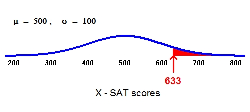
Suppose we are interested in knowing the probability that a randomly selected student will score 633 or more on the math portion of his or her SAT (this is represented by the red area). Again, 633 does not fall exactly 1, 2, or 3 standard deviations above the mean. Notice, however, that an SAT score of 633 and a foot length of 13 are both about 1/3 of the way between 1 and 2 standard deviations.
Finding Probabilities for a Normal Random Variable
As we saw, the Standard Deviation Rule is very limited in helping us answer probability questions, and basically limited to questions involving values that fall exactly 1, 2, and 3 standard deviations away from the mean. How do we answer probability questions in general? The key is the position of the value relative to the mean, measured in standard deviations.
We can approach the answering of probability questions two possible ways: a table and technology. In the next sections, you will learn how to use the "standard normal table," and then how the same calculations can be done with technology.
Standardizing Values : The first step to assessing a probability associated with a normal value is to determine the relative value with respect to all the other values taken by that normal variable. This is accomplished by determining how many standard deviations below or above the mean that value is.
Example: Foot Length
How many standard deviations below or above the mean male foot length is 13 inches? Since the mean is 11 inches, 13 inches is 2 inches above the mean. Since a standard deviation is 1.5 inches, this would be 2 / 1.5 = 1.33 standard deviations above the mean. Combining these two steps, we could write:
(13 in. - 11 in.) / (1.5 inches per standard deviation) = (13 - 11) / 1.5 standard deviations = +1.33 standard deviations.
In the language of statistics, we have just found the z-score for a male foot length of 13 inches to be z = +1.33. Or, to put it another way, we have standardized the value of 13. In general, the standardized value z tells how many standard deviations below or above the mean the original value is, and is calculated as follows:
z-score = (value - mean)/standard deviation
The convention is to denote a value of our normal random variable X with the letter "x." Since the mean is written \( \mu \) and the standard deviation \( \sigma \), we may write the standardized value as
\( z = \frac{x - \mu}{\sigma} \)
Notice that since \( \sigma \) is always positive, for values of x above the mean \( \mu \), z will be positive; for values of x below \( \mu \), z will be negative.

Example: Standardizing Foot Measurements
Let's go back to our foot length example, and answer some more questions.
(a) What is the standardized value for a male foot length of 8.5 inches? How does this foot length relate to the mean?
z = (8.5 - 11) / 1.5 = -1.67. This foot length is 1.67 standard deviations below the mean.
(b) A man's standardized foot length is +2.5. What is his actual foot length in inches? If z = +2.5, then his foot length is 2.5 standard deviations above the mean. Since the mean is 11, and each standard deviation is 1.5, we get that the man's foot length is: 11 + 2.5(1.5) = 14.75 inches.
z-scores also allow us to compare values of different normal random variables. Here is an example:
(c) In general, women's foot length is shorter than men's. Assume that women's foot length follows a normal distribution with a mean of 9.5 inches and standard deviation of 1.2. Ross' foot length is 13.25 inches, and Candace's foot length is only 11.6 inches. Which of the two has a longer foot relative to his or her gender group?
To answer this question, let's find the z-score of each of these two normal values, bearing in mind that each of the values comes from a different normal distribution.
Ross: z-score = (13.25 - 11) / 1.5 = 1.5 (Ross' foot length is 1.5 standard deviations above the mean foot length for men).
Candace: z-score = (11.6 - 9.5) / 1.2 = 1.75 (Candace's foot length is 1.75 standard deviations above the mean foot length for women).
Note that even though Ross' foot is longer than Candace's, Candace's foot is longer relative to their respective genders.
- Explanation :
Indeed, Tom's z-score = (22.50-27)/4 = -1.125
- Explanation :
Indeed, a z-score of 1.125 indicates that Tom’s hourly rate of $22.50 is 1.125 standard deviations below the mean score.
- Explanation :
Indeed, John's z-score is 2.6 standard deviations above the mean, which is much above average. In particular, from the standard deviation rule, we know that,since John's z-score is more than 2 standard deviations above the mean, his hourly rate is in the highest 2.5% of salaries.
- Explanation :
Indeed, John's z-score of 2.6 indicates that his salary is 2.6 standard deviations above the mean. Since the mean is $27 and each standard deviation is $4, we get that John's salary = 27 + 2.6(4) = $37.40.
- Explanation :
Indeed, Cindy's z-score is -2, while Tom’s z-score is (22.50-27) / 4 = -1.125. Cindy’s hourly salary is lower, since she scored 2 standard deviations below the mean, while Tom scored only 1.125 standard deviations below the mean.
- Explanation :
Indeed, Ron's z-score = (88 - 82) / 5 = 1.2.
- Explanation :
Indeed, a z-score of 1.2 indicates that Ron's score of 88 is 1.2 standard deviations above the mean score.
- Explanation :
Indeed, Dan's z-score indicates that his score is 2.4 standard deviations below the mean, which is much below average. In particular, from the standard deviation rule, we know that, since Dan's score is less than 2 standard deviations below the mean, his score is in the lowest 2.5% of scores.
- Explanation :
Indeed, Dan's z-score of -2.4 indicates that his score is 2.4 standard deviations below the mean. Since the mean is 82 and each standard deviation is 5, we get that Dan's score = 82 - 2.4(5) = 70
- Explanation :
Indeed, Ron's z-score is 1.2, and Julie's z-score is (84 - 75) / 6 = 1.5. Julie's score is more impressive, since she scored 1.5 standard deviations above the mean, while Ron scored only 1.2 standard deviations above the mean.
Standard Normal Table: Introduction
Now that you have learned to assess the relative value of any normal value by standardizing, the next step is to evaluate probabilities.
In other contexts, as mentioned before, we will first take the conventional approach of referring to a normal table, which tells the probability of a normal variable taking a value less than any standardized score z.
Since normal curves are symmetric about their mean, it follows that the curve of z scores must be symmetric about 0.
Since the total area under any normal curve is 1, it follows that the areas on either side of z = 0 are both 0.5.
Also, according to the Standard Deviation Rule, most of the area under the standardized curve falls between z = -3 and z = +3.
The normal table outlines the precise behavior of the standard normal random variable Z, the number of standard deviations a normal value x is below or above its mean. The normal table provides probabilities that a standardized normal random variable Z would take a value less than or equal to a particular value z*.
These particular values are listed in the form *.* in rows along the left margins of the table, specifying the ones and tenths. The columns fine-tune these values to hundredths, allowing us to look up the probability of being below any standardized value z of the form *.**. Here is part of the table.
z .00 .01 .02 .03 .04 .05 .06 .07 .08 .09 -3.4 .0003 .0003 .0003 .0003 .0003 .0003 .0003 .0003 .0003 .0002 -3.3 .0005 .0005 .0005 .0004 .0004 .0004 .0004 .0004 .0004 .0003 -3.2 .0007 .0007 .0006 .0006 .0006 .0006 .0006 .0005 .0005 .0005 -3.1 .0010 .0009 .0009 .0009 .0008 .0008 .0008 .0008 .0007 .0007 -3.0 .0013 .0013 .0013 .0012 .0012 .0011 .0011 .0011 .0010 .0010 -2.9 .0019 .0018 .0018 .0017 .0016 .0016 .0015 .0015 .0014 .0014 -2.8 .0026 .0025 .0024 .0023 .0023 .0022 .0021 .0021 .0020 .0019 -2.7 .0035 .0034 .0033 .0032 .0031 .0030 .0029 .0028 .0027 .0026 -2.6 .0047 .0045 .0044 .0043 .0041 .0040 .0039 .0038 .0037 .0036 -2.5 .0062 .0060 .0059 .0057 .0055 .0054 .0052 .0051 .0049 .0048 -2.4 .0082 .0080 .0078 .0075 .0073 .0071 .0069 .0068 .0066 .0064 -2.3 .0107 .0104 .0102 .0099 .0096 .0094 .0091 .0089 .0087 .0084 -2.2 .0139 .0136 .0132 .0129 .0125 .0122 .0119 .0116 .0113 .0110 -2.1 .0179 .0174 .0170 .0166 .0162 .0158 .0154 .0150 .0146 .0143 -2.0 .0228 .0222 .0217 .0212 .0207 .0202 .0197 .0192 .0188 .0183 -1.9 .0287 .0281 .0274 .0268 .0262 .0256 .0250 .0244 .0239 .0233 -1.8 .0359 .0351 .0344 .0336 .0329 .0322 .0314 .0307 .0301 .0294 -1.7 .0446 .0436 .0427 .0418 .0409 .0401 .0392 .0384 .0375 .0367 -1.6 .0548 .0537 .0526 .0516 .0505 .0495 .0485 .0475 .0465 .0455 -1.5 .0668 .0655 .0643 .0630 .0618 .0606 .0594 .0582 .0571 .0559 -1.4 .0808 .0793 .0778 .0764 .0749 .0735 .0721 .0708 .0694 .0681 -1.3 .0968 .0951 .0934 .0918 .0901 .0885 .0869 .0853 .0838 .0823 -1.2 .1151 .1131 .1112 .1093 .1075 .1056 .1038 .1020 .1003 .0985 -1.1 .1357 .1335 .1314 .1292 .1271 .1251 .1230 .1210 .1190 .1170 -1.0 .1587 .1562 .1539 .1515 .1492 .1469 .1446 .1423 .1401 .1379 -0.9 .1841 .1814 .1788 .1762 .1736 .1711 .1685 .1660 .1635 .1611 -0.8 .2119 .2090 .2061 .2033 .2005 .1977 .1949 .1922 .1894 .1867 -0.7 .2420 .2389 .2358 .2327 .2296 .2266 .2236 .2206 .2177 .2148 -0.6 .2743 .2709 .2676 .2643 .2611 .2578 .2546 .2514 .2483 .2451 -0.5 .3085 .3050 .3015 .2981 .2946 .2912 .2877 .2843 .2810 .2776 -0.4 .3446 .3409 .3372 .3336 .3300 .3264 .3228 .3192 .3156 .3121 -0.3 .3821 .3783 .3745 .3707 .3669 .3632 .3594 .3557 .3520 .3483 -0.2 .4207 .4168 .4129 .4090 .4052 .4013 .3974 .3936 .3897 .3859 -0.1 .4602 .4562 .4522 .4483 .4443 .4404 .4364 .4325 .4286 .4247 -0.0 .5000 .4960 .4920 .4880 .4840 .4801 .4761 .4721 .4681 .4641 z .00 .01 .02 .03 .04 .05 .06 .07 .08 .09 0.0 .5000 .5040 .5080 .5120 .5160 .5199 .5239 .5279 .5319 .5359 0.1 .5398 .5438 .5478 .5517 .5557 .5596 .5636 .5675 .5714 .5753 0.2 .5793 .5832 .5871 .5910 .5948 .5987 .6026 .6064 .6103 .6141 0.3 .6179 .6217 .6255 .6293 .6331 .6368 .6406 .6443 .6480 .6517 0.4 .6554 .6591 .6628 .6664 .6700 .6736 .6772 .6808 .6844 .6879 0.5 .6915 .6950 .6985 .7019 .7054 .7088 .7123 .7157 .7190 .7224 0.6 .7257 .7291 .7324 .7357 .7389 .7422 .7454 .7486 .7517 .7549 0.7 .7580 .7611 .7642 .7673 .7704 .7734 .7764 .7794 .7823 .7852 0.8 .7881 .7910 .7939 .7967 .7995 .8023 .8051 .8078 .8106 .8133 0.9 .8159 .8186 .8212 .8238 .8264 .8289 .8315 .8340 .8365 .8389 1.0 .8413 .8438 .8461 .8485 .8508 .8531 .8554 .8577 .8599 .8621 1.1 .8643 .8665 .8686 .8708 .8729 .8749 .8770 .8790 .8810 .8830 1.2 .8849 .8869 .8888 .8907 .8925 .8944 .8962 .8980 .8997 .9015 1.3 .9032 .9049 .9066 .9082 .9099 .9115 .9131 .9147 .9162 .9177 1.4 .9192 .9207 .9222 .9236 .9251 .9265 .9279 .9292 .9306 .9319 1.5 .9332 .9345 .9357 .9370 .9382 .9394 .9406 .9418 .9429 .9441 1.6 .9452 .9463 .9474 .9484 .9495 .9505 .9515 .9525 .9535 .9545 1.7 .9554 .9564 .9573 .9582 .9591 .9599 .9608 .9616 .9625 .9633 1.8 .9641 .9649 .9656 .9664 .9671 .9678 .9686 .9693 .9699 .9706 1.9 .9713 .9719 .9726 .9732 .9738 .9744 .9750 .9756 .9761 .9767 2.0 .9772 .9778 .9783 .9788 .9793 .9798 .9803 .9808 .9812 .9817 2.1 .9821 .9826 .9830 .9834 .9838 .9842 .9846 .9850 .9854 .9857 2.2 .9861 .9864 .9868 .9871 .9875 .9878 .9881 .9884 .9887 .9890 2.3 .9893 .9896 .9898 .9901 .9904 .9906 .9909 .9911 .9913 .9916 2.4 .9918 .9920 .9922 .9925 .9927 .9929 .9931 .9932 .9934 .9936 2.5 .9938 .9940 .9941 .9943 .9945 .9946 .9948 .9949 .9951 .9952 2.6 .9953 .9955 .9956 .9957 .9959 .9960 .9961 .9962 .9963 .9964 2.7 .9965 .9966 .9967 .9968 .9969 .9970 .9971 .9972 .9973 .9974 2.8 .9974 .9975 .9976 .9977 .9977 .9978 .9979 .9979 .9980 .9981 2.9 .9981 .9982 .9982 .9983 .9984 .9984 .9985 .9985 .9986 .9986 3.0 .9987 .9987 .9987 .9988 .9988 .9989 .9989 .9989 .9990 .9990 3.1 .9990 .9991 .9991 .9991 .9992 .9992 .9992 .9992 .9993 .9993 3.2 .9993 .9993 .9994 .9994 .9994 .9994 .9994 .9995 .9995 .9995 3.3 .9995 .9995 .9995 .9996 .9996 .9996 .9996 .9996 .9996 .9997 3.4 .9997 .9997 .9997 .9997 .9997 .9997 .9997 .9997 .9997 .9998 By construction, the probability P(Z < z*) equals the area under the z curve to the left of that particular value z*.
A quick sketch is often the key to solving normal problems easily and correctly.
Standard Normal Table: Finding a Probability
(a) What is the probability of a normal random variable taking a value less than 2.8 standard deviations above its mean? According to the table, P(Z < 2.8) = 0.9974 or 99.74%.
z .00 .01 .02 .03 .04 .05 .06 .07 .08 .09 2.5 .9938 .9940 .9941 .9943 .9945 .9946 .9948 .9949 .9951 .9952 2.6 .9953 .9955 .9956 .9957 .9959 .9960 .9961 .9962 .9963 .9964 2.7 .9965 .9966 .9967 .9968 .9969 .9970 .9971 .9972 .9973 .9974 2.8 .9974 .9975 .9976 .9977 .9977 .9978 .9979 .9979 .9980 .9981 2.9 .9981 .9982 .9982 .9983 .9984 .9984 .9985 .9985 .9986 .9986 3.0 .9987 .9987 .9987 .9988 .9988 .9989 .9989 .9989 .9990 .9990 
(b) What is the probability of a normal random variable taking a value lower than 1.47 standard deviations below its mean? P(Z < -1.47) = 0.0708, or 7.08%.
z .00 .01 .02 .03 .04 .05 .06 .07 .08 .09 -1.5 .0668 .0655 .0643 .0630 .0618 .0606 .0594 .0582 .0571 .0559 -1.4 .0808 .0793 .0778 .0764 .0749 .0735 .0721 .0708 .0694 .0681 -1.3 .0968 .0951 .0934 .0918 .0901 .0885 .0869 .0853 .0838 .0823 -1.2 .1151 .1131 .1112 .1093 .1075 .1056 .1038 .1020 .1003 .0985 
(c) What is the probability of a normal random variable taking a value more than 0.75 standard deviations above its mean?
The fact that the problem involves the word "more" rather than "less" should not be overlooked! Our normal table, like most, provides left-tail probabilities, and adjustments must be made for any other type of problem.
Method 1: By symmetry of the z curve centered on 0, P(Z > +0.75) = P(Z < -0.75) = 0.2266.
Method 2: Because the total area under the normal curve is 1,
P(Z > +0.75) = 1 - P(Z < +0.75) = 1 - 0.7734 = 0.2266.
[Note: most students prefer to use Method 1, which does not require subtracting 4-digit probabilities from 1.]
(d) What is the probability of a normal random variable taking a value between 1 standard deviation below and 1 standard deviation above its mean?
To find probabilities in between two standard deviations, we must put them in terms of the probabilities below. A sketch is especially helpful here:
P(-1 < Z < +1) = P(Z < +1) - P(Z < -1) = 0.8413 - 0.1587 = 0.6826
- Explanation :
Indeed, P(Z < 1.05) is just the table 's entry for z = 1.05, which is 0.8531.
- Explanation :
Indeed, P(-1.5 < Z < 2.5) = P(Z < 2.5) - P(Z < -1.5) = 0.9938 - 0.0668 = 0.9270.
- Explanation :
Indeed, P(Z > 2.55) = P(Z < -2.55) = .0054 or, P(Z > 2.55) = 1 - P(Z < 2.55) = 1 - .9946 = 0.0054.
Standard Normal Table: Finding a z Value
So far, we have used the normal table to find a probability, given the number (z) of standard deviations below or above the mean.
The solution process involved first locating the given z value of the form *.** in the margins, then finding the corresponding probability of the form .**** inside the table as our answer.
Now, in Example 2, a probability will be given and we will be asked to find a z value.
The solution process involves first locating the given probability of the form .**** inside the table, then finding the corresponding z value of the form *.** as our answer.
Example :
The probability is 0.01 that a standardized normal variable takes a value below what particular value of z?
The closest we can come to a probability of 0.01 inside the table is 0.0099, in the z = -2.3 row and .03 column: z = -2.33. In other words, the probability is 0.01 that the value of a normal variable is lower than 2.33 standard deviations below its mean.
z .00 .01 .02 .03 .04 .05 .06 .07 .08 .09 -2.5 .0062 .0060 .0059 .0057 .0055 .0054 .0052 .0051 .0049 .0048 -2.4 .0082 .0080 .0078 .0075 .0073 .0071 .0069 .0068 .0066 .0064 -2.3 .0107 .0104 .0102 .0099 .0096 .0094 .0091 .0089 .0087 .0084 -2.2 .0139 .0136 .0132 .0129 .0125 .0122 .0119 .0116 .0113 .0110 -2.1 .0179 .0174 .0170 .0166 .0162 .0158 .0154 .0150 .0146 .0143 
The probability is 0.15 that a standardized normal variable takes a value above what particular value of z?
Remember that the table only provides probabilities of being below a certain value, not above. Once again, we must rely on one of the properties of the normal curve to make an adjustment.
Method 1: According to the table, 0.15 (actually 0.1492) is the probability of being below -1.04. By symmetry, 0.15 must also be the probability of being above +1.04.
z .00 .01 .02 .03 .04 .05 .06 .07 .08 .09 -1.2 .1151 .1131 .1112 .1093 .1075 .1056 .1038 .1020 .1003 .0985 -1.1 .1357 .1335 .1314 .1292 .1271 .1251 .1230 .1210 .1190 .1170 -1.0 .1587 .1562 .1539 .1515 .1492 .1469 .1446 .1423 .1401 .1379 -0.9 .1841 .1814 .1788 .1762 .1736 .1711 .1685 .1660 .1635 .1611 -0.8 .2119 .2090 .2061 .2033 .2005 .1977 .1949 .1922 .1894 .1867 
Method 2: If 0.15 is the probability of being above the value we seek, then 1 - 0.15 = 0.85 must be the probability of being below the value we seek. According to the table, 0.85 (actually 0.8508) is the probability of being below +1.04.
In other words, we have found 0.15 to be the probability that a normal variable takes a value more than 1.04 standard deviations above its mean.
(c) The probability is 0.95 that a normal variable takes a value within how many standard deviations of its mean?
A symmetric area of 0.95 centered at 0 extends to values -z* and +z* such that the remaining (1 - .95) / 2 = 0.025 is below -z* and also 0.025 above +z*. The probability is 0.025 that a standardized normal variable is below -1.96. Thus, the probability is 0.95 that a normal variable takes a value within 1.96 standard deviations of its mean. Once again, the Standard Deviation Rule is shown to be just roughly accurate, since it states that the probability is 0.95 that a normal variable takes a value within 2 standard deviations of its mean.
Comment : Our standard normal table, like most, only provides probabilities for z values between -3.49 and +3.49. The following example demonstrates how to handle cases where z exceeds 3.49 in absolute value.
Example : (a) What is the probability of a normal variable being lower than 5.2 standard deviations below its mean?
There is no need to panic about going "off the edge" of the normal table. We already know from the Standard Deviation Rule that the probability is only about (1 - .997) / 2 = 0.0015 that a normal value would be more than 3 standard deviations away from its mean in one direction or the other. The table provides information for z values as extreme as plus or minus 3.49: the probability is only .0002 that a normal variable would be lower than 3.49 standard deviations below its mean. Any more standard deviations than that, and we generally say the probability is approximately zero.
In this case, we would say the probability of being lower than 5.2 standard deviations below the mean is approximately zero:
P(Z < -5.2) = 0 (approx.)
(b) What is the probability of the value of a normal variable being higher than 6 standard deviations below its mean?
Since the probability of being lower than 6 standard deviations below the mean is approximately zero, the probability of being higher than 6 standard deviations below the mean must be approximately 1. P(Z > -6) = 1 (approx.)
(c) What is the probability of a normal variable being less than 8 standard deviations above the mean? Approximately 1. P(Z < +8) = 1 (approx.)
(d) What is the probability of a normal variable being greater than 3.5 standard deviations above the mean? Approximately 0. P(Z > +3.5) = 0 (approx.)
- Explanation :
Indeed, P(Z > 2.17) = 0.015.
Standard Normal Table: Working with Non-standard Normal Values
"How likely or unlikely is a male foot length of more than 13 inches?" We were unable to solve the problem, because 13 inches didn't happen to be one of the values featured in the Standard Deviation Rule. Subsequently, we learned how to standardize a normal value (tell how many standard deviations below or above the mean it is) and how to use the normal table to find the probability of falling in an interval a certain number of standard deviations below or above the mean. By combining these two skills, we will now be able to answer questions like the one above.
Example: Male Foot Length Male foot lengths have a normal distribution, with \( \mu = 11; \sigma = 1.5 \) inches. What is the probability of a foot length of more than 13 inches?
First, we standardize: \( z = \frac{x - \mu}{\sigma} = \frac{13-11}{15} = +1.33 \) ; the probability that we seek, P(X > 13), is the same as the probability
P(Z > +1.33) that a normal variable takes a value greater than 1.33 standard deviations above its mean.
This can be solved with the normal table, after applying the property of symmetry:
P(Z > +1.33) = P(Z < -1.33) = 0.0918. A male foot length of more than 13 inches is on the long side, but not too unusual: its probability is about 9%.
Comment: We can streamline the solution in terms of probability notation. Since the standardized value for 13 is (13 - 11) / 1.5 = +1.33, we can write \( P(X > 13) = P(Z > 1.33) =P(Z < -1.33) =0.0918 \).
The first equality above holds because we subtracted the mean from a normal variable X and divided by its standard deviation, transforming it to a standardized normal variable that we call "Z."
The second equality above holds by the symmetry of the standard normal curve around zero.
The last equality above was obtained from the normal table.
What is the probability of a male foot length between 10 and 12 inches?
The standardized values of 10 and 12 are, respectively, \( \frac{10-11}{1.5} = -0.67 ; \frac{12 - 11}{1.5} = 0.67 \)
P(-.67 < Z < +.67) = P(Z < +.67) - P(Z < -.67) = .7486 - .2514 = 0.4972.
Or, if you prefer the streamlined notation, \( P(10 < X < 12) = P(-0.67 < Z < +0.67) = P(Z < +0.67) - P(Z < -0.67) = 0.7486 - 0.2514 = 0.4972\)
Comment : By solving the above example, we inadvertently discovered the quartiles of a normal distribution! P(Z < -0.67) = 0.2514 tells us that roughly 25%, or one quarter, of a normal variable's values are less than 0.67 standard deviations below the mean. P(Z < +0.67) = 0.7486 tells us that roughly 75%, or three quarters, are less than .67 standard deviations above the mean. And of course the median is equal to the mean, since the distribution is symmetric, the median is 0 standard deviations away from the mean.
Example: Length of a Human Pregnancy Length (in days) of a randomly chosen human pregnancy is a normal random variable with \( \mu = 266; \sigma = 16 \) Find Q1, the median, and Q3. Q1 = 266 - 0.67(16) = 255; median = mean = 266;
Q3 = 266 + 0.67(16) = 277. Thus, the probability is 1/4 that a pregnancy will last less than 255 days; 1/2 that it will last less than 266 days; 3/4 that it will last less than 277 days.
What is the probability that a randomly chosen pregnancy will last less than 246 days? Since (246 - 266) / 16 = -1.25, we write
\( P(X < 246) = P(Z < -1.25) = 0.1056 \)
What is the probability that a randomly chosen pregnancy will last longer than 240 days? Since (240 - 266) / 16 = -1.63, we write
\( P(X > 240) = P(Z > -1.63) = P(Z < +1.63) = 0.9484 \)
Since the mean is 266 and the standard deviation is 16, most pregnancies last longer than 240 days.
What is the probability that a randomly chosen pregnancy will last longer than 500 days?
Method 1 : Common sense tells us that this would be impossible.
Method 2 : The standardized value of 500 is (500 - 266) / 16 = +14.625. \( P(X > 500) = P(Z > 14.625) = 0\).
Suppose a pregnant woman's husband has scheduled his business trips so that he will be in town between the 235th and 295th days. What is the probability that the birth will take place during that time? The standardized values are (235 - 266) / 16) = -1.94 and (295 - 266) / 16 = +1.81.
\( P(235 < X < 295) = P(-1.94 < Z < +1.81) = P(Z < +1.81) - P(Z < -1.94) = 0.9649 - 0.0262 = 0.9387 \)
There is close to a 94% chance that the husband will be in town for the birth.
Solved Questions : Scenario: SAT Math Scores
According to the College Board website, the scores on the math part of the SAT (SAT-M) in a certain year had a mean of 507 and standard deviation of 111. Assume that SAT scores follow a normal distribution. What is the probability that a randomly chosen student (from all those taking the SAT-M that year) scored above 700? In other words, what proportion of students who took the SAT scored above 700? Yet another, more technical way to ask this question is: what is P(X > 700), where X represents the random variable SAT-M score?
We are given that the random variable X representing the SAT-M score has a normal distribution with a mean of 507 and a standard deviation of 111, and we are asked to find P(X > 700). The z-score of 700 is (700 - 507) / 111 = 1.74 (rounded), and therefore:
P(X > 700) = P(Z > 1.74) = (by symmetry) P(Z < -1.74) = (using the table) 0.0409.
We conclude that roughly 4.1% of the students score above 700 on the SAT-M.
What proportion of students score between 400 and 600 on the SAT-M? In other words, find P(400 < X < 600).
We need to find P(400 < X < 600), where X is a normal random variable with a mean of 507 and a standard deviation of 111.
The z-score of 400 is (400 - 507)/111 = -.96 (rounded).
The z-score of 600 is (600 - 507)/111 = .84 (rounded), and therefore,
P(400 < X < 600) = P(-.96 < Z < .84) = P(Z < .84) - P(Z < -.96) = (table) .7995 - .1685 = 0.6310
We conclude that roughly 63.1% of the students score between 400 and 600.
Standard Normal Table: Finding an X value
The previous examples all followed the same general form: given values of a normal random variable, you were asked to find an associated probability. The two basic steps in the solution process were to
standardize to Z; and
find associated probabilities inside the normal table.
The next example will be a different type of problem: given a certain probability, you will be asked to find the associated value of the normal random variable. The solution process will go more or less in reverse order from what it was in the previous examples.
Example: Foot Length Revisited Again, foot length of a randomly chosen adult male is a normal random variable with a mean of 11 and standard deviation of 1.5.
The probability is 0.04 that a randomly chosen adult male foot length will be less than how many inches?
According to the normal table, a probability of 0.04 below (actually 0.0401) is associated with z = -1.75
In other words, the probability is 0.04 that a normal variable takes a value lower than 1.75 standard deviations below its mean. For adult male foot lengths, this would be 11 - 1.75(1.5) = 8.375. The probability is 0.04 that an adult male foot length would be less than 8.375 inches.
The probability is 0.10 that an adult male foot will be longer than how many inches? Caution is needed here because of the word "longer." Once again, we must remind ourselves that the table only shows the probability of a normal variable taking a value lower than a certain number of standard deviations below or above its mean. Adjustments must be made for problems that involve probabilities besides "lower than" or "less than." As usual, we have a choice of invoking either symmetry or the fact that the total area under the normal curve is 1. Students should examine both methods and decide which they prefer to use for their own purposes.
Method 1: According to the table, a probability of 0.10 below is associated with a z value of -1.28. By symmetry, it follows that a probability of 0.10 above has z = +1.28. We seek the foot length that is 1.28 standard deviations above its mean: 11 + 1.28(1.5) = 12.92, or just under 13 inches.
Method 2: If the probability is 0.10 that a foot will be longer than the value we seek, then the probability is 0.90 that a foot will be shorter than that same value, since the probabilities must sum to 1.
According to the table, a probability of .90 below is associated with a z value of +1.28. Again, we seek the foot length that is 1.28 standard deviations above its mean, or 12.92 inches.
Comment Part (a) in the above example could have been re-phrased as:
"0.04 is the proportion of all adult male foot lengths that are below what value?", which takes the perspective of thinking about the probability as a proportion of occurrences in the long-run. As originally stated, it focuses on the chance of a randomly chosen individual having a normal value in a given interval.
Example: Money Spent for Lunch A study reported that the amount of money spent each week for lunch by a worker in a particular city is a normal random variable with a mean of $35 and a standard deviation of $5.
The probability is 0.97 that a worker will spend less than how much money in a week on lunch?
The z associated with a probability of 0.9700 below is +1.88. The amount that is 1.88 standard deviations above the mean is 35 + 1.88(5) = 44.4, or $44.40.
There is a 30% chance of spending more than how much for lunches in a week?
The z associated with a probability of 0.30 above is +0.52. The amount is 35 + 0.52(5) = 37.6, or $37.60.
Comment Another way of expressing Example (part a.) above would be to ask, "What is the 97th percentile for the amount (X) spent by workers in a week for their lunch?" Many normal variables, such as heights, weights, or exam scores, are often expressed in terms of percentiles.
Example The height X (in inches) of a randomly chosen woman is a normal random variable with a mean of 65 and a standard deviation of 2.5. What is the height of a woman who is in the 80th percentile? A probability of 0.7995 in the table corresponds to z = +.84. Her height is 65 + .84(2.5) = 67.1 inches.
By now we have had practice in solving normal probability problems in both directions: those where a normal value is given and we are asked to report a probability, and those where a probability is given and we are asked to report a normal value. Strategies for solving such problems are outlined below:
Steps in Solving Two Types of Normal Problems Given a normal value x, solve for probability:
Standardize: calculate \( z = \frac{x - \mu}{\sigma} \)
Locate z in the margins of the normal table (ones and tenths for the row, hundredths for the column). Find the corresponding probability (given to four decimal places) of a normal random variable taking a value below z inside the table. (Adjust if the problem involves something other than a "less-than" probability, by invoking either symmetry or the fact that the total area under the normal curve is 1.)
Given a probability, solve for normal value x:
(Adjust if the problem involves something other than a "less-than" probability, by invoking either symmetry or the fact that the total area under the normal curve is 1.) Locate the probability (given to four decimal places) inside the normal table. Find the corresponding z value in the margins (row for ones and tenths, column for hundredths).
"Unstandardize": calculate \( x = \mu + z * \sigma \).
Scenario: SAT Math Scores
According to the College Board website, the scores on the math part of the SAT (SAT-M) in a certain year had a mean of 507 and standard deviation of 111. Assume that SAT scores follow a normal distribution.
One of the criteria for admission to a certain engineering school is an SAT-M score in the top 2% of scores. How does this translate to an actual SAT-M score? In other words, how high must a student score on the SAT-M in order for his application to be considered? A different way to ask the same question is "What is the 98th percentile of the SAT-M distribution?"
- Explanation :
We are looking for the value x, so that P(X > x) = 0.02. The same value also satisfies P(X < x) = 0.98. This way of posing the problem works best for us, since our table is set up to work with "less than" rather than "greater than".
- Explanation :
The closest probability of 0.98 is 0.9798. Looking at the margins, we see that this probability corresponds to a z-score of 2.05. This means that in order to be in the top 2% of SAT-M scores (and thus be considered for the engineering school) a student must score more than 2.05 standard deviations above the mean.
- Explanation :
In order to be in the top 2% of SAT-M scores (and thus be considered for the engineering school) a student must score more than 2.05 standard deviations above the mean. 2.05 standard deviations above the mean is a score of 507 + 2.05(111) = 734.55. Since SAT-M scores are whole numbers, we conclude that in order to be considered for the engineering school a student must have an SAT-M score of at least 735.
Q. Scenario: Adult Male Height Adult male height (X) follows (approximately) a normal distribution with a mean of 69 inches and a standard deviation of 2.8 inches. Using a statistical package, we find the following probabilities: P(X < 65) = 0.07656373 P(X < 75) = 0.98393771
What proportion of males are less than 65 inches tall? Round your answer to TWO decimal places ? 0.08
What proportion of males are more than 75 inches tall? Round your answer to TWO decimal places ? 0.02; The proportion of males that are more than 75 inches tall is equal to 1 - 0.98393771 which equals 0.01606229 and rounds to 0.02.
Q. Scenario: Adult Male Height Adult male height (X) follows (approximately) a normal distribution with a mean of 69 inches and a standard deviation of 2.8 inches. Using a statistical package, we find the following the value for x that satisfies P(X < x) P(X < x) = 0.005, x = 61.78768 P(X < x) = 0.9975, x = 76.8597
How tall must a male be, in order to be among the tallest 0.25% of males? Round your answer to ONE decimal place. There proportion for men *less* than 76.9 is 0.9975, so the proportion of males *greater* than 76.9 is 0.0025.