• Application of Normal Random Variables: Approximation to Binomial One of the important applications of the normal distribution is that under certain conditions it can provide a very good approximation to the binomial distribution. We've seen before that sometimes calculating binomial probabilities can be quite tedious, and the solution we suggested before is to use statistical software to do the work for you. In the absence of statistical software, another solution would be to use the normal approximation (when appropriate). Normal calculations never get too complicated; all we have to do is use a table correctly. Let's start with a motivating example. Example: True/False Questions Suppose a student answers 20 true/false questions completely at random. What is the probability of getting no more than 8 correct? Let X be the number of questions the student gets right (successes) out of the 20 questions (trials), when the probability of success is .5. X is therefore a binomial random variable with n = 20 and p = .5, and we are looking for \( P(X \leq 8) = P(X = 0) + P(X = 1) + ... + P(X = 8) \). Doing this by hand using the binomial distribution formula is very tedious, and requires us to do 9 complex calculations, as shown below: \( \frac{20!}{0!20!} 0.5^0(1-0.5)^{20-0} + \frac{20!}{1!19!} 0.5^1(1-0.5)^{20-1} + ... + \frac{20!}{8!12!} 0.5^8(1-0.5)^{20-8} = 0.2517\) One option that we have is to use statistical software, which will provide the answer:

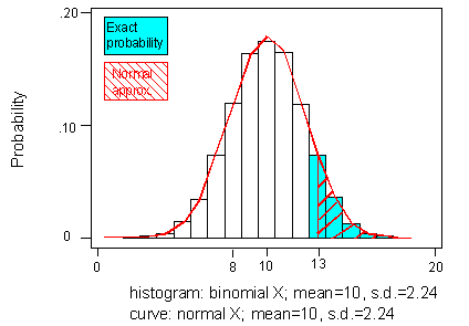
• Consider the appearance of the probability histogram for the distribution of X:




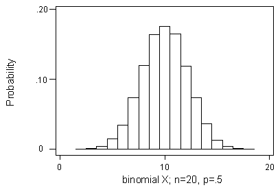
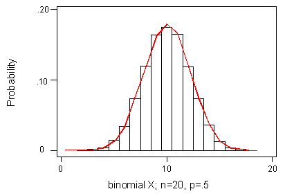
• Clearly, the shape of the distribution of X for n = 20, p = 0.5 has a normal appearance: symmetric, bulging at the middle, and tapering at the ends. The following figure should help you visualize this:




• This suggests a method of approximating binomial probabilities:




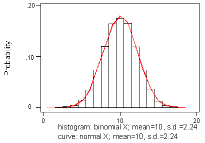
• Estimate the binomial probability of X_B taking a value over a certain interval with the probability that a normal random variable X_N takes a value over the same interval, where X_N has the same mean and standard deviation as X_B, namely \( \mu = np ; \sigma = \sqrt{np(1-p)}




• Example Suppose a student answers 20 true/false questions completely at random. Use a normal approximation to estimate the probability of getting no more than 8 correct. The number (X) correct is a binomial random variable that represents the number of successes in 20 trials when the probability of success for each trial is 0.5. X has a mean and standard deviation of:




• \( \mu = np = 20*0.5 = 10; \sigma = \sqrt{np(1-p) = \sqrt{20*0.5*(1-0.5)} = 2.24}




• and so we approximate the binomial X with a normal random variable having the same mean and standard deviation: Then we solve in the usual way using normal tables:




• \( P(X_B \leq 8) \sim P(X_N \leq 8) = P(Z \leq \frac{8-10}{2.24}) = P(Z \leq -0.89) = 0.1867\)




• Unfortunately, the approximated probability, .1867, is quite a bit different from the actual probability, 0.2517.

Rule of Thumb

• Probabilities for a binomial random variable X with n and p may be approximated by those for a normal random variable having the same mean and standard deviation as long as the sample size n is large enough relative to the proportions of successes and failures, p and 1 - p. Our Rule of Thumb will be to require that \( np \geq 10; n(1-p) \geq 10 \)




• Example May we use a normal approximation for a binomial X with n = 20 and p = 0.5? In this case, np = 20(.5) = 10 and n(1 - p) = 20(1 - .5) = 10. The criteria are just barely satisfied, and so we should not expect the approximation to be especially good.




• The purpose of the next activity is to give you practice at deciding whether the normal approximation is appropriate for a given binomial random variable. You'll get to practice checking the rule of thumb \( np \geq 10; n(1-p) \geq 10 \) , but also get a visual sense of when the normal approximation is appropriate.

View Answer


View Answer


View Answer


View Answer

Q. Recall that when appropriate, a binomial random variable can be approximated by a normal random variable that has the same mean and standard deviation as the binomial random variable. In other words, when appropriate, a binomial random variable with n trials and probability of success p, can be approximated by a normal distribution with mean μ = np and standard deviation σ = sqrt( np (1 - p) ). For those binomial distributions in questions 1-4 above of the previous exercise for which the normal approximation is appropriate, write down which normal distribution you would use to approximate them.

• For example 1:




1. X is binomial with n = 100 and p = 0.75, and would therefore be approximated by a normal random variable having mean μ = 100 * 0.75 = 75 and standard deviation σ = sqrt(100 * 0.75 * 0.25) = sqrt(18.75) = 4.33.




2. Note that if you look at the histogram, this makes sense.




3. The distribution is indeed centered at 75, and extends approximately 3 standard deviations (3 * 4.33 = 13) on each side of the mean (as we know normal distributions do).




• For example 4:




1. X is binomial with n = 300 and p = .9, 0 and would therefore be approximated by a normal random variable having mean μ = 300 * 0.9 = 270 and standard deviation σ = sqrt(300 * 0.9 * 0.1) = sqrt(27) = 5.2.




2. Note that if you look at the histogram, this makes sense.




3. The distribution is indeed centered at 270, and extends approximately 3 standard deviations (3 * 5.2 = 15.6) on each side of the mean (as we know normal distributions do).

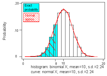
• It is possible to improve the normal approximation to the binomial by adjusting for the discrepancy that arises when we make the shift from the areas of histogram rectangles to the area under a smooth curve. For example, if we want to find the binomial probability that X is less than or equal to 8, we are including the area of the entire rectangle over 8, which actually extends to 8.5. Our normal approximation only included the area up to 8. The figure below illustrates this:




• It can be improved upon by making the continuity correction:




• in this case, we would have




• \( P(X_B \leq 8) \sim P(X_N \leq 8.5) = P(Z \leq \frac{8.5 - 10}{2.24}) = P(Z \leq -0.67) = 0.2514 \)




• , which is much closer to the actual binomial probability of 0.2517 than our original approximation (0.1867) was.




• Similarly, suppose I wanted to answer: What is the probability that the student gets at least 13 questions right?




• Here, to calculate the exact probability we are including the area of the entire rectangle over 13, which actually starts from 12.5. Our normal approximation only included the area from 13. The continuity correction in this case would be:




• \( P(X_B \geq 13) \sim P(X_N \geq 12.5) = P(Z \leq \frac{12.5 - 10}{2.24}) = P(Z \geq 1.12) = P(Z \leq -1.12) = 0.1314 \)




• It turns out that the exact probability in this case (using software) is 0.1316, so the approximation is excellent.




• The purpose of the next activity is to give you guided practice in solving word problems involving a binomial random variable, when the normal approximation is appropriate and is extremely helpful.

Scenario: Left-Handed College Students

• Roughly 10% of all college students in the United States are left-handed. Most academic institutions, therefore, try to have at least a few left-handed chairs in each classroom. 225 students are about to enter a lecture hall that has 30 left-handed chairs for a lecture. What is the probability that this is not going to be enough; in other words, what is the probability that more than 30 (or at least 31) of the 225 students are left-handed?




• Let X be the number of left-handed students (success) out of the 225 students (trials). X is therefore binomial with n = 225 and p = 0.1. We are asked to find P(X > 30) or P(X ≥ 31). Explain why we can use the normal approximation in this case, and state which normal distribution you would use for the approximation.




1. X is binomial with n = 225 and p = 0.1. The normal approximation is appropriate, since the rule of thumb is satisfied: np = 225 * 0.1 = 22.5 > 10, and also n(1 - p) = 225 * 0.9 = 202.5 > 10.




2. We will approximate the binomial random variable X by the random variable Y having a normal distribution with mean μ = 225 * 0.1 = 22.5 and standard deviation σ = sqrt(225 * 0.1 * 0.9) = sqrt(20.25) = 4.5




• Use the normal approximation to find P(X ≥ 31). For the approximation to be better, use the continuity correction as we did in the last example. In other words, rather than approximating P(X ≥ 31) by P(Y ≥ 31), approximate it by P(Y ≥ 30.5).




1. P(X ≥ 31) ≈ (normal approximation + continuity correction) ≈ P(Y ≥ 30.5) = P(Z ≥ (30.5 - 22.5) / 4.5) = P(Z ≥ 1.78) = (symmetry) = P(Z ≤ -1.78) = (table) = 0.0375.

• Already on several occasions we have pointed out the important distinction between a population and a sample.




• In Exploratory Data Analysis, we learned to summarize and display values of a variable for a sample, such as displaying the blood types of 100 randomly chosen adults using a pie chart, or displaying the heights of 150 males using a histogram and supplementing it with the sample mean \( \overline{X} \) and sample standard deviation (S).




• In our study of Probability and Random Variables, we discussed the long-run behavior of a variable, considering the population of all possible values taken by that variable.




• For example, we talked about the distribution of blood types among all adults and the distribution of the random variable X, representing a male's height.




• In this module, we focus directly on the relationship between the values of a variable for a sample and its values for the entire population from which the sample was taken.




• This module is the bridge between probability and our ultimate goal of the course, statistical inference. In inference, we look at a sample and ask what we can say about the population from which it was drawn.




• In this module, we'll pose the reverse question: If I know what the population looks like, what can I expect the sample to look like?




• Clearly, inference poses the more practical question, since in practice we can look at a sample, but rarely do we know what the whole population looks like. This module will be more theoretical in nature, since it poses a problem which is not really practical, but will present important ideas which are the underpinnings for statistical inference.

• Example: Example #1: Blood Type




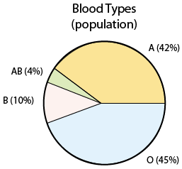
1. In the probability section, we presented the distribution of blood types in the entire U.S. population:




2. 




3. Assume now that we take a sample of 500 people in the United States, record their blood type, and display the sample results:




4. 




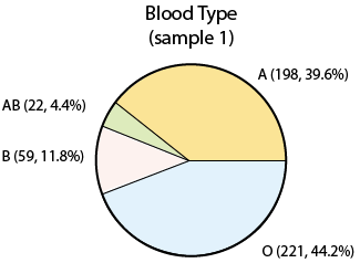
5. Note that the percentages (or proportions) that we got in our sample are slightly different than the population percentages. This is really not surprising. Since we took a sample of just 500, we cannot expect that our sample will behave exactly like the population, but if the sample is random (as it was), we expect to get results which are not that far from the population (as we did). If we took yet another sample of size 500:




6. 




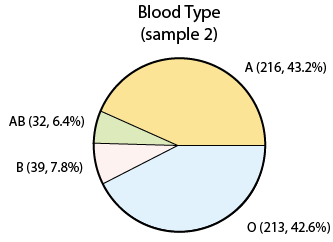
7. we again get sample results that are slightly different from the population figures, and also different from what we got in the first sample. This very intuitive idea, that sample results change from sample to sample, is called sampling variability.




• Example: Example #2: Heights of Adult Males




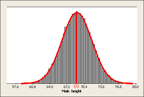
1. Heights among the population of all adult males follow a normal distribution with a mean \( \mu = 69 \) inches and a standard deviation \( \sigma = 2.8 \) inches. Here is a probability display of this population distribution:




2. 




3. A sample of 200 males was chosen, and their heights were recorded. Here are the sample results:




4. 




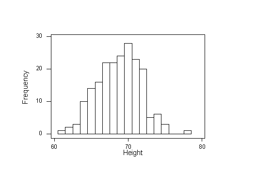
5. The sample mean is \( \overline{x} = 68.7 \) inches and the sample standard deviation is s = 2.95 inches.




6. Again, note that the sample results are slightly different from the population. The histogram we got resembles the normal distribution, but is not as fine, and also the sample mean and standard deviation are slightly different from the population mean and standard deviation. Let's take another sample of 200 males:




7. 




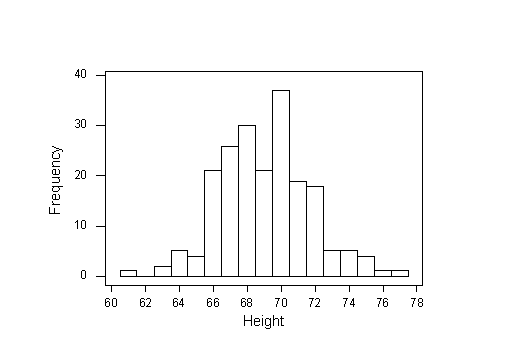
8. The sample mean is \( \overline{x} = 69.065 \) inches and the sample standard deviation is s = 2.659 inches.




• Again, as in Example 1 we see the idea of sampling variability. Again, the sample results are pretty close to the population, and different from the results we got in the first sample.




• In both the examples, we have numbers that describe the population, and numbers that describe the sample. In Example 1, the number 42% is the population proportion of blood type A, and 39.6% is the sample proportion (in sample 1) of blood type A. In Example 2, 69 and 2.8 are the population mean and standard deviation, and (in sample 1) 68.7 and 2.95 are the sample mean and standard deviation.




• parameter and statistic (definition) A parameter is a number that describes the population; a statistic is a number that is computed from the sample.




1. In Example 1: 42% is the parameter and 39.6% is a statistic.




2. In Example 2: 69 and 2.8 are the parameters and 68.7 and 2.95 are the statistics.




• In this course, as in the examples above, we focus on the following parameters and statistics:




• population proportion and sample proportion




• population mean and sample mean




• population standard deviation and sample standard deviation




• The following table summarizes the three pairs, and gives the notation




• 	(Population) Parameter	(Sample) Statistic
  Proportion	\( p \)	\( \hat{p} \)
  Mean	\( \mu \)	\( \overline{x} \)
  Standard Deviation	\( \sigma \)	\( s \)




• The only new notation here is p for population proportion (p = 0.42 for type A in Example 1), and \( \hat{p} \) for sample proportion




• ( \( \hat{p} \) = 0.396 for type A in Example 1).




• Comments




1. Parameters are usually unknown, because it is impractical or impossible to know exactly what values a variable takes for every member of the population.




2. Statistics are computed from the sample, and vary from sample to sample due to sampling variability.




• In the last part of the course, statistical inference, we will learn how to use a statistic to draw conclusions about an unknown parameter, either by estimating it or by deciding whether it is reasonable to conclude that the parameter equals a proposed value. In this module, we'll learn about the behavior of the statistics assuming that we know the parameters. So, for example, if we know that the population proportion of blood type A in the population is 0.42, and we take a random sample of size 500, what do we expect the sample proportion \( \hat{p} \) to be?




• Example If students picked numbers completely at random from the numbers 1 to 20, the proportion of times that the number 7 would be picked is .05. When 15 students picked a number "at random" from 1 to 20, 3 of them picked the number 7. Identify the parameter and accompanying statistic in this situation.




1. The parameter is the population proportion of random selections resulting in the number 7, which is p = 0.05. The accompanying statistic is the sample proportion of selections resulting in the number 7, which is \( \hat{p} = 3/15 = 0.2 \).




• Example The length of human pregnancies has a mean of 266 days and a standard deviation of 16 days. A random sample of 9 pregnant women was observed to have a mean pregnancy length of 270 days, with a standard deviation of 14 days. Identify the parameters and accompanying statistics in this situation.




1. The parameters are population mean \( \mu = 266 \) and population standard deviation \( \sigma = 16 \). The accompanying statistics are sample mean \( \overline{x} = 270 \) and sample standard deviation s = 14.

• The SAT-Verbal scores of a sample of 300 students at a particular university had a mean of 592 and standard deviation of 73. According to the university's reports, the SAT-Verbal scores of all its students had a mean of 580 and a standard deviation of 110.

View Answer



View Answer



View Answer



View Answer



View Answer



View Answer

• The first step to drawing conclusions about parameters based on the accompanying statistics is to understand how sample statistics behave relative to the parameter that summarizes the entire population




• Behavior of Sample Proportion \( \hat{p} \)




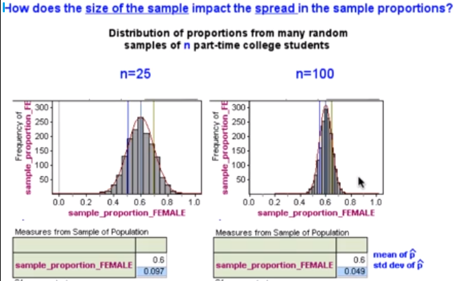
1. Approximately 60% of all part-time college students in the United States are female. (In other words, the population proportion of females among part-time college students is p = 0.6.) What would you expect to see in terms of the behavior of a sample proportion of females \( \hat{p} \) if random samples of size 100 were taken from the population of all part-time college students?




2. As we saw before, due to sampling variability, sample proportion in random samples of size 100 will take numerical values which vary according to the laws of chance: in other words, sample proportion is a random variable. To summarize the behavior of any random variable, we focus on three features of its distribution: the center, the spread, and the shape.




3. Based only on our intuition, we would expect the following:




1. Center: Some sample proportions will be on the low side—say, 0.55 or 0.58—while others will be on the high side—say, 0.61 or 0.66. It is reasonable to expect all the sample proportions in repeated random samples to average out to the underlying population proportion, .6. In other words, the mean of the distribution of \( \hat{p} \) should be p.




2. Spread: For samples of 100, we would expect sample proportions of females not to stray too far from the population proportion 0.6. Sample proportions lower than 0.5 or higher than 0.7 would be rather surprising. On the other hand, if we were only taking samples of size 10, we would not be at all surprised by a sample proportion of females even as low as 4/10 = 0.4, or as high as 8/10 = 0.8. Thus, sample size plays a role in the spread of the distribution of sample proportion: there should be less spread for larger samples, more spread for smaller samples.




3. Shape: Sample proportions closest to 0.6 would be most common, and sample proportions far from 0.6 in either direction would be progressively less likely. In other words, the shape of the distribution of sample proportion should bulge in the middle and taper at the ends: it should be somewhat normal.




4. Comment




1. The distribution of the values of the sample proportions \( \hat{p} \) in repeated samples is called the sampling distribution of \( \hat{p} \).




2. The purpose of the next activity is to check whether our intuition about the center, spread and shape of the sampling distribution of \( \hat{p} \) was right via simulations.

• We're going to discuss the behavior of sample proportions by investigating these two questions:




1. when we collect random samples what patterns emerge?




2. More specifically, what is the shape, center, and spread of the distribution of sample proportions?




• To investigate these questions we're going to return to the familiar context of the previous example and look at the population of all part-time college students.




• We're assuming that sixty percent of this population is female.




• Now what we're going to be investigating in this movie is what happens as we begin to take random samples from this population.




• I'm going to be collecting random samples of 25 students at a time.




• Each random sample will have a different proportion of females. What we're interested in is what is going to happen when we began to collect many random samples.




• While we run the simulation, Each sample had 25 part-time college students in it and for each sample I calculated the proportion that were female and I recorded that here.




• What looks like happened over the long run is that many of the samples had proportions that were close to the population proportion of 0.6.




• We can also see that as we moved further away from 0.6 we had fewer samples with sample proportions in that range.




• 




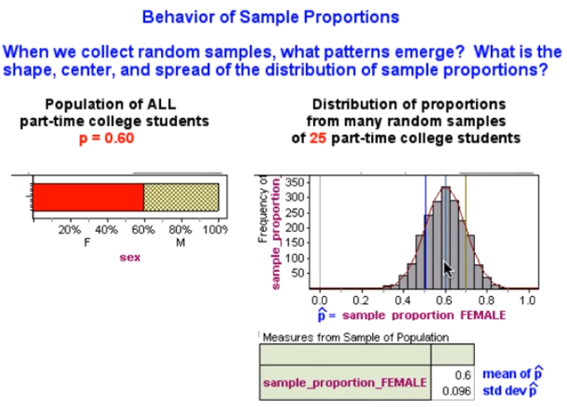
• We can get a more accurate sense of the variability in sample proportions by looking at the standard deviation. Here the standard deviation is roughly 10%.




• That tells me that typical samples had proportions that fell between about 0.5 and 0.7. Here in the graph I have marked one standard deviation below and one standard deviation above the mean of 0.6.




• Another thing we notice is that the shape is approximately normal. I have used a mathematical formula here to graph a normal curve on top of the sampling distribution and we can see that the normal distribution models the sample proportions well. This is encouraging.




• It tells me that a normal model will be a good probability model for the sampling distribution of sample proportions.




• 




• When I increased the sample size by a factor of four, the standard deviation decreased to about half of what it was previously. So, I can conclude that larger samples do have less variability.




• I also notice that the mean of the sampling distribution stayed at 0.6. So the mean does not seem to be impacted by sample size. I also see that the distribution is normal for this case.

View Answer



View Answer



View Answer

• If repeated random samples of a given size n are taken from a population of values for a categorical variable, where the proportion in the category of interest is p, then the mean of all sample proportions \( \hat{p} \) is the population proportion (p).




• As for the spread of all sample proportions, theory dictates the behavior much more precisely than saying that there is less spread for larger samples. In fact, the standard deviation of all sample proportions \( \hat{p} \) is exactly \( \sqrt{\frac{p(1-p)}{n}} \).




• Since sample size n appears in the denominator of the square root, the standard deviation does decrease as sample size increases. Finally, the shape of the distribution of \( \hat{p} \) will be approximately normal as long as the sample size n is large enough. The convention is to require both np and n(1 - p) to be at least 10.




• We can summarize all of the above by the following:




• \( \hat{p} \) has a normal distribution with a mean of \( \mu_{\hat{p}} = p\) and standard deviation \( \sigma_{\hat{p}} = \sqrt{\frac{p(1-p)}{n}}\) (and as long as np and n(1 - p) are at least 10).




• Let's apply this result to our example and see how it compares with our simulation.




• In our example, n = 25 (sample size) and p = 0.6. Note that np = 15 ≥ 10 and n(1 - p) = 10 ≥ 10. Therefore we can conclude that \( \hat{p} \) is approximately a normal distribution with mean p = 0.6 and standard deviation \( \sqrt{\frac{p(1-p)}{n}} = \sqrt{\frac{0.6(1-0.6)}{25}} = 0.097\) (which is very close to what we saw in our simulation).

Scenario: Student Loans

• According to the National Postsecondary Student Aid Study conducted by the U.S. Department of Education in 2008, 62% of graduates from public universities had student loans.




• We randomly sample college graduates from public universities and determine the proportion in the sample with student loans.

View Answer



View Answer



View Answer



View Answer



View Answer



View Answer

• The proportion of left-handed people in the general population is about 0.10. To simulate this population, we constructed a collection in which p = 0.10. We then conducted four simulations, drawing random samples of different sizes from this collection. Here you see the resulting sampling distributions and corresponding summary tables:




• 




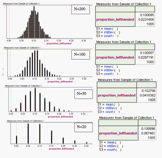
• Explain how these simulations illustrate the theory discussed above.




• Shape: Theory tells us that if np ≥ 10 and n(1 - p) ≥ 10, then the sampling distribution is approximately normal. When p = 0.10, these conditions are not met for n = 20 or n = 50. We can see that the distributions are skewed to the right for these sample sizes. As the sample size increases, we see the distributions becoming more normal. For n = 100 and for larger samples, the conditions are met, and we see that a normal distribution is a pretty good model for the sampling distribution.




• Note: We only collected 1,005 samples. The theory presumes we have collected all possible samples. So we don't expect the simulations to give perfectly normal distributions.




• Center: All of the sampling distributions are centered at approximately p = 0.10.




• Spread: The standard deviation of each sampling distribution is very close to the value predicted by




• \( \sqrt{\frac{p(1-p)}{n}} \)




• For example, using this formula for n = 20, the standard deviation is predicted to be 0.0671. We see in the simulation that the standard deviation is 0.0675, which is very close to the predicted value.

• A random sample of 100 students is taken from the population of all part-time students in the United States, for which the overall proportion of females is 0.6.




• (a) There is a 95% chance that the sample proportion \( \hat{p} \) falls between what two values? First note that the distribution of has the mean p = 0.6, standard deviation \( \sqrt{\frac{p(1-p)}{n}} = \sqrt{\frac{0.6(1-0.6)}{100}} = 0.05\), and a shape that is close to normal, since np = 100(0.6) = 60 and n(1 - p) = 100(0.4) = 40 are both greater than 10. The Standard Deviation Rule applies: the probability is approximately 0.95 that \( \hat{p} \) falls within 2 standard deviations of the mean, that is, between 0.6 - 2(0.05) and 0.6 + 2(0.05). There is roughly a 95% chance that \( \hat{p} \) falls in the interval (0.5, 0.7).




• (b) What is the probability that sample proportion \( \hat{p} \) is less than or equal to 0.56?




• To find P(\( \hat{p} \leq 0.56\) ), we standardize 0.56 to z = (0.56 - 0.60) /0.05 = -0.80:




• P(\( \hat{p} \leq 0.56\) ) = P(Z ≤ -0.8) = 0.2119

• A random sample of 2,500 students is taken from the population of all part-time students in the United States, for which the overall proportion of females is 0.6.




• (a) There is a 95% chance that the sample proportion \( \hat{p} \) falls between what two values? First note that the distribution of \( \hat{p} \) has the mean p = 0.6, standard deviation \( \sqrt{\frac{p(1-p)}{n}} = \sqrt{\frac{0.6(1-0.6)}{2500}} = 0.01\), and a shape that is close to normal, since np = 2500(0.6) = 1500 and n(1 - p) = 2500(0.4) = 1000 are both greater than 10. The standard deviation rule applies: the probability is approximately 0.95 that \( \hat{p} \) falls within 2 standard deviations of the mean, that is, between 0.6 - 2(0.01) and 0.6 + 2(0.01). There is roughly a 95% chance that \( \hat{p} \) falls in the interval (0.58, 0.62).




• (b) What is the probability that sample proportion \( \hat{p} \) is less than 0.56?




• To find P(\( \hat{p} \) ≤ 0.56) , we standardize 0.56 to z = (0.56 - 0.60) / 0.01 = -4.00:




• P(\( \hat{p} \) ≤ 0.56) = P(Z ≤ -4.0) = 0, approximately.

• As long as the sample is truly random, the distribution of \( \hat{p} \) is centered at p, no matter what size sample has been taken.




• Larger samples have less spread.




• Specifically, when we multiplied the sample size by 25, increasing it from 100 to 2,500, the standard deviation was reduced to 1/5 of the original standard deviation.




• Sample proportion strays less from population proportion 0.6 when the sample is larger: it tends to fall anywhere between 0.5 and 0.7 for samples of size 100, whereas it tends to fall between 0.58 and 0.62 for samples of size 2,500.




• It is not so improbable to take a value as low as 0.56 for samples of 100 (probability is more than 20%) but it is almost impossible to take a value as low as low as 0.56 for samples of 2,500 (probability is virtually zero).




• The purpose of this next activity is to give guided practice in finding the sampling distribution of the sample proportion




• (\( \hat{p} \)), and use it to draw conclusions about what values of \( \hat{p} \) we are most likely to get.

• The proportion of left-handed people in the general population is about 0.1. Suppose a random sample of 225 people is observed. What is the sampling distribution of the sample proportion (p̂ )? In other words, what can we say about the behavior of the different possible values of the sample proportion that we can get when we take such a sample? (Note: normal approximation is valid because 0.1(225) = 22.5 and 0.9(225) = 202.5 are both more than 10.)




1. The possible values of the sample proportion follow approximately a normal distribution with mean p = 0.1, and standard deviation =\( \sqrt{\frac{p(1-p)}{n}} = \sqrt{\frac{0.1(1-0.1)}{225}} = 0.02\)




• Since the sample proportion has a normal distribution, its values follow the Standard Deviation Rule. What interval is almost certain (probability 0.997) to contain the sample proportion of left-handed people?




1. Since the Standard Deviation Rule applies, the probability is approximately 0.997 that the sample proportion falls within 3 standard deviations of its mean, that is, between 0.1 - 3(0.02) and 0.1 + 3(0.02). There is roughly a 99.7% chance, therefore, that the sample proportion falls in the interval (0.04, 0.16).




• In a sample of 225 people, would it be unusual to find that 40 people in the sample are left-handed?




1. About 18% (40/225) of this sample is left-handed. In the previous problem, we determined that there is roughly a 99.7% chance that a sample proportion will fall between 0.04 and 0.16. So a sample proportion of 0.18 is very unlikely. Note: According to the Standard Deviation Rule, sample proportions greater than 0.16 will occur 0.15% of the time. (100% - 99.7%) / 2 = 0.15%.




• Find the approximate probability of at least 27 in 225 (proportion 0.12) being left-handed. In other words, what is P(p̂ ≥ 0.12)? Guidance: Note that 0.12 is exactly 1 standard deviation (0.02) above the mean (0.1). Now use the Standard Deviation Rule.




1. Note that 0.12 is exactly 1 standard deviation above the mean. The Standard Deviation Rule tells us that there is a 68% chance that the sample proportion falls within 1 standard deviation of its mean, that is, between 0.08 and 0.12. There is therefore a probability of (1 - 0.68) / 2 = 0.16 that the sample proportion falls above 0.12.

• We are now moving on to explore the behavior of the statistic \( \overline{X} \), the sample mean, relative to the parameter \( \mu \), the population mean (when the variable of interest is quantitative).




• Example




1. Birth weights are recorded for all babies in a town. The mean birth weight is 3,500 grams, µ = 3,500 g. If we collect many random samples of 9 babies at a time, how do you think sample means will behave?




2. Here again, we are working with a random variable, since random samples will have means that vary unpredictably in the short run but exhibit patterns in the long run.




3. Based on our intuition and what we have learned about the behavior of sample proportions, we might expect the following about the distribution of sample means:




4. Center: Some sample means will be on the low side—say 3,000 grams or so—while others will be on the high side—say 4,000 grams or so. In repeated sampling, we might expect that the random samples will average out to the underlying population mean of 3,500 g. In other words, the mean of the sample means will be µ, just as the mean of sample proportions was p.




5. Spread: For large samples, we might expect that sample means will not stray too far from the population mean of 3,500. Sample means lower than 3,000 or higher than 4,000 might be surprising. For smaller samples, we would be less surprised by sample means that varied quite a bit from 3,500. In others words, we might expect greater variability in sample means for smaller samples. So sample size will again play a role in the spread of the distribution of sample measures, as we observed for sample proportions.




6. Shape: Sample means closest to 3,500 will be the most common, with sample means far from 3,500 in either direction progressively less likely. In other words, the shape of the distribution of sample means should bulge in the middle and taper at the ends with a shape that is somewhat normal. This, again, is what we saw when we looked at the sample proportions.




7. Comment The distribution of the values of the sample mean \( \overline{x} \) in repeated samples is called the sampling distribution of \( \overline{x} \).

• If repeated random samples of a given size n are taken from a population of values for a quantitative variable, where the population mean is \( \mu \) and the population standard deviation is \( \sigma \), then the mean of all sample means \( \overline{x} \) is population mean \( \mu \). As for the spread of all sample means, theory dictates the behavior much more precisely than saying that there is less spread for larger samples. In fact, the standard deviation of all sample means \( \overline{x} \) is exactly \( \frac{\sigma}{\sqrt{n}} \). Since the square root of sample size n appears in the denominator, the standard deviation does decrease as sample size increases.




• Scenario: Pell Grant Awards




1. The Federal Pell Grant Program provides need-based grants to low-income undergraduate and certain postbaccalaureate students to promote access to postsecondary education. According to the National Postsecondary Student Aid Study conducted by the U.S. Department of Education in 2008, the average Pell grant award for 2007-2008 was $2,600. Assume that the standard deviation in Pell grant awards was $500.




2. If we randomly sample 36 Pell grant recipients and record the mean Pell grant award for the sample, then repeat the sampling process many, many times, what is the mean and standard deviation of the sample means?




3. The distribution of sample means will have a mean equal to μ = 2,600 and a standard deviation of - \( \frac{\sigma}{\sqrt{n}} = \frac{500}{\sqrt{36} = 83.3 \)




4. The population mean for Verbal IQ scores is 100, with a standard deviation of 15. Suppose a researcher takes 50 random samples, with 30 people in each sample. What is mean of the sample means?




5. The mean of the sample means is the population mean; therefore, the mean of the sample means or the sampling distribution of the mean is 100.




6. What is the standard deviation of the sample means? The standard deviation of the sample means is calculated by dividing the population standard deviation by the square root of the sample size; therefore, σ/sqrt(n) = 15/sqrt(30)= 15/5.48= 2.74.

• Variable	Parameter	Statistic	Center	Spread	Shape
  Categorical (example: left-handed or not)	p = population proportion	\( \hat{p} \) = sample proportion	p	\( \sqrt{\frac{p(1-p)}{n}} \)	Normal IF np ≥ 10 and n(1 - p) ≥ 10
  Quantitative (example: age)	μ = population mean, σ = population standard deviation	\( \overline{x} \) = sample mean	\( \mu \)	\( \frac{\sigma}{\sqrt{n}} \)	Normal if n > 30 (always normal if population is normal)




• If a variable is skewed in the population and we draw small samples, the distribution of sample means will be likewise skewed. If we increase the sample size to around 30 (or larger), the distribution of sample means becomes approximately normal.




• To summarize, the distribution of sample means will be approximately normal as long as the sample size is large enough. This discovery is probably the single most important result presented in introductory statistics courses. It is stated formally as the Central Limit Theorem.




• We will depend on the Central Limit Theorem again and again in order to do normal probability calculations when we use sample means to draw conclusions about a population mean. We now know that we can do this even if the population distribution is not normal.




• How large a sample size do we need in order to assume that sample means will be normally distributed? Well, it really depends on the population distribution, as we saw in the simulation. The general rule of thumb is that samples of size 30 or greater will have a fairly normal distribution regardless of the shape of the distribution of the variable in the population.




• Comment: For categorical variables, our claim that sample proportions are approximately normal for large enough n is actually a special case of the Central Limit Theorem.

• Recall our earlier scenario: The Federal Pell Grant Program provides need-based grants to low-income undergraduate and certain postbaccalaureate students to promote access to postsecondary education. According to the National Postsecondary Student Aid Study conducted by the U.S. Department of Education in 2008, the average Pell grant award for 2007-2008 was $2,600. Assume that the standard deviation in Pell grants awards was $500.

View Answer



View Answer

• Household size in the United States has a mean of 2.6 people and standard deviation of 1.4 people.




• (a) What is the probability that a randomly chosen household has more than 3 people?




1. A normal approximation should not be used here, because the distribution of household sizes would be considerably skewed to the right. We do not have enough information to solve this problem.




• (b) What is the probability that the mean size of a random sample of 10 households is more than 3?




1. By anyone's standards, 10 is a small sample size. The Central Limit Theorem does not guarantee sample mean coming from a skewed population to be approximately normal unless the sample size is large.




• (c) What is the probability that the mean size of a random sample of 100 households is more than 3?




1. Note: To review how to determine probabilities for z scores, please refer to the Standard Normal Table section of the Random Variables module.




2. Now we may invoke the Central Limit Theorem: even though the distribution of household size X is skewed, the distribution of sample mean household size \(\overline{X} \) is approximately normal for a large sample size such as 100. Its mean is the same as the population mean, 2.6, and its standard deviation is the population standard deviation divided by the square root of the sample size: \( \frac{\sigma}{\sqrt{n}} = \frac{1.4}{\sqrt{100}} = 0.14\) The z-score for 3 is \( \frac{3-2.6}{\frac{1.4}{\sqrt{100}}} = \frac{0.4}{0.14} = 2.86 \) The probability of the mean household size in a sample of 100 being more than 3 is therefore P(\(\overline{X} \) > 3) = P(Z > 2.86) = P(Z < -2.86) = 0.0021.




3. Households of more than 3 people are, of course, quite common, but it would be extremely unusual for the mean size of a sample of 100 households to be more than 3.

• The annual salary of teachers in a certain state X has a mean of $54,000 and standard deviation of σ = $5,000.




• What is the probability that the mean annual salary of a random sample of 5 teachers from this state is more than $60,000? Find this probability or explain why you cannot.




1. Recall from the Exploratory Data Analysis unit that salary distribution is typically skewed to the right. Since 5 is a small sample size, and the Central Limit Theorem does not guarantee that the sample mean coming from a skewed population is approximately normal unless the sample size is larger, we thus do not have enough information to solve the problem.

View Answer



View Answer



View Answer



View Answer

Scores on the math portion of the SAT (SAT-M) in a recent year have followed a normal distribution with mean μ = 507 and standard deviation σ = 111. What is the probability that the mean SAT-M score of a random sample of 4 students who took the test that year is more than 600? Explain why you can solve this problem, even though the sample size (n = 4) is very low.

• Since the scores on the SAT-M in the population follow a normal distribution, the sample mean automatically also follows a normal distribution, for any sample size. Therefore, the mean has a normal distribution with the same mean as the population, 507, and standard deviation




• \( \frac{\sigma}{\sqrt{n}} = \frac{111}{\sqrt{4}} = 55.5 \)




• The z-score of 600 is therefore:




• \( \frac{600-507}{111/\sqrt{4}} = \frac{93}{55.5} = 1.68 \)




• And therefore,




• \( P(\overline{X} > 600) = P(Z > 1.68) = P(Z < -1.68) = 0.0465 \)




• We find that while it is very common to find students who score above 600 on the SAT-M, it would be quite unlikely (4.65% chance) for the mean score of a sample of 4 students to be above 600.

Previous

Next