• Use a sample to infer (or draw conclusions) about the population from which it was drawn.




• The specific form of inference called for depends on the type of variables involved—either a single categorical or quantitative variable, or a combination of two variables whose relationship is of interest.




• 




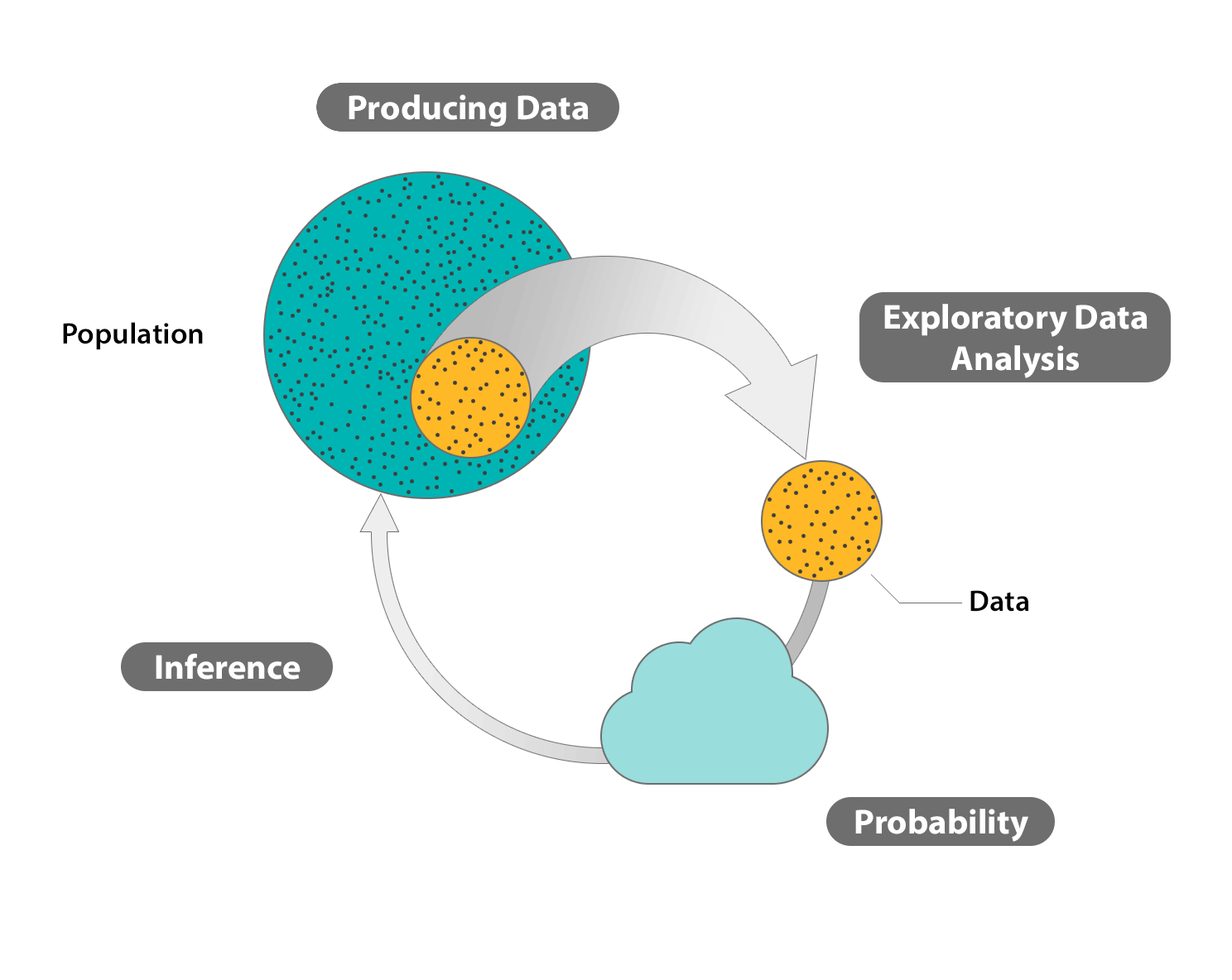
• In the Exploratory Data Analysis sections, we learned to display and summarize data that were obtained from a sample.




• Regardless of whether we had one variable and we examined its distribution, or whether we had two variables and we examined the relationship between them, it was always understood that these summaries applied only to the data at hand; we did not attempt to make claims about the larger population from which the data were obtained.




• Such generalizations were, however, a long-term goal from the very beginning of the course.




• For this reason, in the Producing Data sections, we took care to establish principles of sampling and study design that would be essential in order for us to claim that, to some extent, what is true for the sample should be also true for the larger population from which the sample originated.




• These principles should be kept in mind throughout this section on statistical inference, since the results that we will obtain will not hold if there was bias in the sampling process, or flaws in the study design under which variables' values were measured.




• Perhaps the most important principle stressed in the Producing Data unit was that of randomization.




• Randomization is essential not only because it prevents bias but also because it permits us to rely on the laws of probability, which is the scientific study of random behavior.




• In the Probability sections, we established basic laws for the behavior of random variables. We ultimately focused on two random variables of particular relevance: the sample mean \( \overline{X} \) and the sample proportion \( \hat{p} \), and the last module of the Probability unit was devoted to exploring their sampling distributions.




• We learned what probability theory tells us to expect from the values of the sample mean and the sample proportion, given that the corresponding population parameters - the population mean (μ) and the population proportion (p)—are known.




• As we mentioned in that section, the value of such results is more theoretical than practical, since in real-life situations we seldom know what is true for the entire population. All we know is what we see in the sample, and we want to use this information to say something concrete about the larger population.




• Probability theory has set the stage to accomplish this: learning what to expect from the value of sample mean, given that population mean takes a certain value, teaches us what to expect from the value of the unknown population mean, given that a particular value of sample mean has been observed.




• Similarly, since we have established how sample proportion behaves relative to population proportion, we will now be able to turn this around and say something about the value of population proportion, based on an observed sample proportion.




• This process—inferring something about the population based on what is measured in the sample—is (as you know) called statistical inference.

• We introduce three forms of statistical inference in this unit, each one representing a different way of using the information obtained in the sample to draw conclusions about the population. These forms are:




1. Point estimation




2. Interval estimation




3. Hypothesis testing




• The difference between them in terms of the type of conclusions they draw about the population based on the sample results.




• In point estimation, we estimate an unknown parameter using a single number that is calculated from the sample data.




1. Example : Based on sample results, we estimate that p, the proportion of all U.S. adults who are in favor of stricter gun control, is 0.6.




• In interval estimation, we estimate an unknown parameter using an interval of values that is likely to contain the true value of that parameter (and state how confident we are that this interval indeed captures the true value of the parameter).




1. Example : Based on sample results, we are 95% confident that p, the proportion of U.S. adults who are in favor of stricter gun control, is between 0.57 and 0.63.




• In hypothesis testing, we have some claim about the population, and we check whether or not the data obtained from the sample provide evidence against this claim.




1. Example: 1 It was claimed that among all U.S. adults, about half are in favor of stricter gun control and about half are against it. In a recent poll of a random sample of 1,200 U.S. adults, 60% were in favor of stricter gun control. This data, therefore, provides some evidence against the claim.




2. Example: 2 It is claimed that among drivers 18-23 years of age (our population) there is no relationship between drunk driving and gender. A roadside survey collected data from a random sample of 5,000 drivers and recorded,their gender and whether they were drunk. The collected data showed roughly the same percent of drunk drivers among males and among females. These data, therefore, do not give us any reason to reject the claim that drunk driving is not related to gender.

View Answer



View Answer



View Answer



View Answer



View Answer



View Answer

• We will make a similar distinction here in Inference. In EDA, the type of variable determined the displays and numerical measures we used to summarize the data.




• In Inference, the type of variable of interest (categorical or quantitative) will determine what population parameter we are going to do inference for.




1. When the variable of interest is categorical, the population parameter that we will infer about is the population proportion (p) associated with that variable. For example, if we are interested in studying opinions about the death penalty among U.S. adults, and thus our variable of interest is "death penalty (in favor/against)," we'll choose a sample of U.S. adults and use the collected data to make an inference about p—the proportion of U.S. adults who support the death penalty.




2. When the variable of interest is quantitative, the population parameter that we infer about is the population mean (μ) associated with that variable. For example, if we are interested in studying the annual salaries in the population of teachers in a certain state, we'll choose a sample from that population and use the collected salary data to make an inference about μ, the mean annual salary of all teachers in that state.

• Point estimation is the form of statistical inference in which, based on the sample data, we estimate the unknown parameter of interest using a single value (hence the name point estimation).




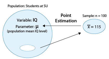
• Example : Suppose that we are interested in studying the IQ levels of students at University (SU)




1. In particular (since IQ level is a quantitative variable), we are interested in estimating μ, the mean IQ level of all the students at Univ.




2. A random sample of 100 SU students was chosen, and their (sample) mean IQ level was found to be \( \overline{x} = 115 \)




3. If we wanted to estimate μ, the population mean IQ level, by a single number based on the sample, it would make intuitive sense to use the corresponding quantity in the sample, the sample mean \( \overline{x} = 115 \).




4. We say that 115 is the point estimate for μ, and in general, we'll always use \( \overline{x} \) as the point estimator for μ.




5. (Note that when we talk about the specific value (115), we use the term estimate, and when we talk in general about the statistic \( \overline{x} \), we use the term estimator. The following figure summarizes this example:




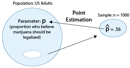
• Example : Opinions of U.S. adults regarding legalizing the use of marijuana




1. In particular, we are interested in the parameter p, the proportion of U.S. adults who believe marijuana should be legalized.




2. Suppose a poll of 1,000 U.S. adults finds that 560 of them believe marijuana should be legalized.




3. If we wanted to estimate p, the population proportion, using a single number based on the sample, it would make intuitive sense to use the corresponding quantity in the sample, the sample proportion \( \hat{p} = \frac{560}{1000} = 0.56 \).




4. We say in this case that 0.56 is the point estimate for p, and in general, we'll always use as \( \hat{p} \) the point estimator for p.




5. (Note, again, that when we talk about the specific value (0.56), we use the term estimate, and when we talk in general about the statistic \( \hat{p} \), we use the term estimator.




6. Here is a visual summary of this example:




7. 

• A study on exercise habits used a random sample of 2,540 college students (1,220 females and 1,320 males).




• The study found the following:




1. 818 of the females in the sample exercise on a regular basis.




2. 924 of the males in the sample exercise on a regular basis.




3. The average time that the 1742 students who exercise on a regular basis (818 + 924) spend exercising per week is 4.2 hours.

View Answer



View Answer



View Answer

Scenario: Newlywed Couples

• A psychology researcher was conducting a study about newlywed heterosexual couples during the first two years of their marriage. 513 newlywed couples were randomly chosen for the study. One of the questions that the researcher was interested in was "During a typical week, how many times do you have sex?" The 513 responses had an average of 2.35 and standard deviation of 1.2. Another question that was asked is "During a typical week, how many evenings do you go out?" 171 of the couples answered that they go out more than twice a week.

View Answer



View Answer

Previous

Next