• Is there a way to increase the precision of the confidence interval (i.e., make it narrower) without compromising on the level of confidence?




• Since the width of the confidence interval is a function of its margin of error, let's look closely at the margin of error of the confidence interval for the mean and see how it can be reduced: \( z* * \frac{\sigma}{\sqrt{n}} \)




• Since z* controls the level of confidence, we can rephrase our question above in the following way:




• Is there a way to reduce this margin of error other than by reducing z*?




• If you look closely at the margin of error, you'll see that the answer is yes. We can do that by increasing the sample size n (since it appears in the denominator).




• Since the margin of error is \( z* * \frac{\sigma}{\sqrt{n}} \), isn't it true that another way to reduce the margin of error (for a fixed z*) is to reduce σ?




1. Answer: While it is true that strictly mathematically speaking the smaller the value of σ, the smaller the margin of error, practically speaking we have absolutely no control over the value of σ (i.e., we cannot make it larger or smaller). σ is the population standard deviation; it is a fixed value (which here we assume is known) that has an effect on the width of the confidence interval (since it appears in the margin of error), but is definitely not a value we can play with.




• Let's try to understand why a larger sample size will reduce the margin of error for a fixed level of confidence. There are three ways to explain it: mathematically, using probability theory, and intuitively.




• We've already alluded to the mathematical explanation; the margin of error is \( z* * \frac{\sigma}{\sqrt{n}} \), and since n, the sample size, appears in the denominator, increasing n will reduce the margin of error.




• As we saw in our discussion about point estimates, probability theory tells us that




• 




• This explains why with a larger sample size the margin of error (which represents how far apart we believe \( \overline{x} \) might be from μ for a given level of confidence) is smaller.




• On an intuitive level, if our estimate \( \overline{x} \) is based on a larger sample (i.e., a larger fraction of the population), we have more faith in it, or it is more reliable, and therefore we need to account for less error around it.




• Comment : While it is true that for a given level of confidence, increasing the sample size increases the precision of our interval estimation, in practice, increasing the sample size is not always possible. Consider a study in which there is a non-negligible cost involved for collecting data from each participant (an expensive medical procedure, for example). If the study has some budgetary constraints, which is usually the case, increasing the sample size from 100 to 400 is just not possible in terms of cost-effectiveness. Another instance in which increasing the sample size is impossible is when a larger sample is simply not available, even if we had the money to afford it. For example, consider a study on the effectiveness of a drug on curing a very rare disease among children. Since the disease is rare, there are a limited number of children who could be participants. This is the reality of statistics. Sometimes theory collides with reality, and you just do the best you can.

View Answer



View Answer

• For a given level of confidence, the sample size determines the size of the margin of error and thus the width, or precision, of our interval estimation. This process can be reversed.




• Example




1. Recall the example about the SAT-M scores of community college students.




2. An educational researcher is interested in estimating μ, the mean score on the math part of the SAT (SAT-M) of all community college students in his state. To this end, the researcher has chosen a random sample of 650 community college students from his state, and found that their average SAT-M score is 475. Based on a large body of research that was done on the SAT, it is known that the scores roughly follow a normal distribution, with the standard deviation \( \sigma = 100\) .




3. The 95% confidence interval for μ is \( 475 - 2*\frac{100}{\sqrt{650}}, 475 + 2*\frac{100}{\sqrt{650}}\), which is roughly \(475 \pm 8\), or (467,484). For a sample size of n = 650, our margin of error is 8.




4. Now, let's think about this problem in a slightly different way:




5. An educational researcher is interested in estimating μ, the mean score on the math part of the SAT (SAT-M) of all community college students in his state with a margin of error of (only) 5, at the 95% confidence level. What is the sample size needed to achieve this? (σ, of course, is still assumed to be 100).




6. To solve this, we set: \( m = 2 * \frac{100}{\sqrt{n}} = 5 \) so \( \sqrt{n} = \frac{2*100}{5} \)




7. and \(n = (\frac{2*100}{5})^2 = 1600 \)




8. So, for a sample size of 1,600 community college students, the researcher will be able to estimate μ with a margin of error of 5, at the 95% level. In this example, we can also imagine that the researcher has some flexibility in choosing the sample size, since there is a minimal cost (if any) involved in recording students' SAT-M scores, and there are many more than 1,600 community college students in each state.




9. Rather than take the same steps to isolate n every time we solve such a problem, we may obtain a general expression for the required n for a desired margin of error m and a certain level of confidence.




10. Since \( m = z*\frac{\sigma}{\sqrt{n}} \) is the formula to determine m for a given n, we can use simple algebra to express n in terms of m (multiply both sides by the square root of n, divide both sides by m, and square both sides) to get \(n = (\frac{z* \sigma}{m})^2 \).




• Comment




1. Clearly, the sample size n must be an integer. In the previous example we got n = 1,600, but in other situations, the calculation may give us a non-integer result. In these cases, we should always round up to the next highest integer.




2. Using this "conservative approach," we'll achieve an interval at least as narrow as the one desired.




• Example




1. IQ scores are known to vary normally with a standard deviation of 15. How many students should be sampled if we want to estimate the population mean IQ at 99% confidence with a margin of error equal to 2?




2. \(n = (\frac{z* \sigma}{m})^2 = (2.576*15/2)^2 = 373.26 \)




3. Round up to be safe, and take a sample of 374 students.

• A study was done on pregnant women who smoke during their pregnancies. In particular, the researchers wanted to study the effect that smoking has on the pregnancy length. A sample 114 pregnant women who were smokers participated in the study and were followed until the birth of their child. At the end of the study, the collected data were analyzed and it was found that the average pregnancy length of the 114 women was 260 days. From a large body of research, it is known that the length of human pregnancy has a standard deviation of 16 days. In the previous activity, we calculated a 95% confidence interval for μ, the mean pregnancy length of women who smoke during their pregnancy based on the given information, and found it to be 260 +/- 3, or (257, 263). Assume now that the researcher wants to get a more precise interval estimation by reducing the margin of error from 3 to 2 while maintaining the same level of confidence. How many additional smoking pregnant women should the researcher sample? (Hint: calculate first what the total sample size must be in order to achieve this).




1. We'll first calculate what the (total) sample size must be in order to get a 95% confidence interval with a margin of error of 2. Using the formula we've developed, we get: \( n = (\frac{2.16}{2})^2 = 256 \) Since the researcher has already collected data from 114 women, the researcher needs to sample 256 - 114 = 142 additional women.




• Comment :




1. In the preceding activity, you saw that in order to calculate the sample size when planning a study, you needed to know the population standard deviation, σ (σ). In practice, σ is usually not known, because it is a parameter. (The rare exceptions are certain variables like IQ score or standardized tests that might be constructed to have a particular known σ.)




2. Therefore, when researchers wish to compute the required sample size in preparation for a study, they use an estimate of σ. Usually, σ is estimated based on the standard deviation obtained in prior studies.




3. However, in some cases, there might not be any prior studies on the topic. In such instances, a researcher still needs to get a rough estimate of the standard deviation of the (yet-to-be-measured) variable, in order to determine the required sample size for the study. One way to get such a rough estimate is with the "range rule of thumb," which you will practice in the following activity.




4. The purpose of the next activity is to give you some experience with a method for roughly estimating σ (σ, the population standard deviation) when no prior studies are available, in order to compute sample size when planning a first study.




• An increasing global population requires more food from crops. With the world's farmland limited due to overuse and a warming globe, one solution may come from crops that are genetically-engineered to grow in harsh desert soil. Suppose that an agricultural researcher has just genetically engineered a brand new type of corn, never before tested, which the researcher hopes will yield a sufficient number of kernels of corn when grown in harsh desert soil. In order to test the corn, the researcher will grow a certain number of ears of the new corn in harsh desert soil, and will count and record the number of kernels per ear. The researcher needs your statistical help in computing the minimum number of ears of the new corn that will be needed to be grown for the study. If the researcher wants to estimate the number of kernels per ear from the experimental corn with a margin of error of m = 80 kernels, with 95% confidence, what is the equation to determine the minimum required number, n, of ears of corn needed in the study, according to what you’ve learned thus far?




1. The formula for the minimum required sample size (in this case number of ears of corn) is n = (2σ / 80)2, where we used z = 2 for 95% confidence.




• In the formula for the required number (n) of ears of corn the researcher needs in the study, you should have seen that we need to know σ. Remember that the variable of interest is the number of kernels per ear of corn; so in this case σ represents the standard deviation of number of kernels (from ear to ear), for the population of all ears of the new genetically engineered corn. In this case, σ (the standard deviation of kernels per ear) isn’t known, since the genetically engineered corn is brand new; and since the new corn has never been tested, there are no prior studies to use to estimate σ. So the researcher can use the ‘range rule of thumb,’ which says that, to a rough approximation, σ is no bigger than range/4, where range = max – min. If you have no other estimate for σ, you can therefore use range/4 as a rough estimate for σ. To use range/4 as a rough estimate for σ, we need to estimate the range of the number of kernels on an ear of the new experimental corn. An ordinary ear of corn has around 800 kernels. We don’t know how few or how many kernels each ear of the experimental corn will have, but at the very minimum it could have zero (if the new corn didn’t produce any kernels at all); and even if the new corn actually over-produces compared to existing corn (despite being grown in harsh conditions), it certainly isn’t going to overproduce by more than twice (since it’s going to be grown in harsh desert soil), so the maximum number of kernels can’t be larger than 1,600.




• Using these common-sense estimates for the max and the min, compute range/4.




1. The range = 1600 so 1600/4 = 400.




• Now, use your previously-computed value as an approximation for sigma, and compute how many ears of the experimental corn the researcher needs in the study.




1. Correct: \( n = (2 x 400 / 80)^2 = (10)^2 = 100 \)

• when the variable that we're interested in studying in the population is categorical, the parameter we are trying to infer about is the population proportion (p) associated with that variable. We also learned that the point estimator for the population proportion p is the sample proportion \( \hat{p} \).




• 




• We are now moving on to interval estimation of p. In other words, we would like to develop a set of intervals that, with different levels of confidence, will capture the value of p. We've actually done all the groundwork and discussed all the big ideas of interval estimation when we talked about interval estimation for μ, so we'll be able to go through it much faster. Let's begin.




• Recall that the general form of any confidence interval for an unknown parameter is: \( estimate \pm margin of error \)




• Since the unknown parameter here is the population proportion p, the point estimator (as I reminded you above) is the sample proportion \( \hat{p} \). The confidence interval for p, therefore, has the form: \( \hat{p} \pm m \)




• (Recall that m is the notation for the margin of error.) The margin of error (m) tells us with a certain confidence what the maximum estimation error is that we are making, or in other words, that \( \hat{p} \) is different from p (the parameter it estimates) by no more than m units.




• From our previous discussion on confidence intervals, we also know that the margin of error is the product of two components: \( m = confidence multiplier . SD of the estimator \)




• To figure out what these two components are, we need to go back to a result we obtained in the Sampling Distributions module of the Probability unit about the sampling distribution of \( \hat{p} \). We found that under certain conditions, \( \hat{p} \) has a normal distribution with mean p, and standard deviation \( \sqrt{\frac{p(1-p)}{n}} \). This result makes things very simple for us, because it reveals what the two components are that the margin of error is made of:




• Since, like the sampling distribution of \( \overline{X} \), the sampling distribution of \( \hat{p} \) is normal, the confidence multipliers that we'll use in the confidence interval for p will be the same z* multipliers we use for the confidence interval for μ when σ is known (using exactly the same reasoning and the same probability results). The multipliers we'll use, then, are: 1.645, 2, and 2.576 at the 90%, 95% and 99% confidence levels, respectively.




• The standard deviation of our estimator \( \hat{p} \) is \( \sqrt{\frac{p(1-p)}{n}} \) Putting it all together, we find that the confidence interval for p should be: \( \hat{p} \pm z*.\sqrt{\frac{p(1-p)}{n}} \). We just have to solve one practical problem and we're done. We're trying to estimate the unknown population proportion p, so having it appear in the confidence interval doesn't make any sense. To overcome this problem,




• We'll replace p with its sample counterpart, \( \hat{p} \), and work with the standard error of \( \hat{p} \), \( \sqrt{\frac{\hat{p}(1-\hat{p})}{n}} \).




• The confidence interval for the population proportion p is: \( \hat{p} \pm z*.\sqrt{\frac{\hat{p}(1-\hat{p})}{n}} \)

• The drug Viagra became available in the U.S. in May, 1998, in the wake of an advertising campaign that was unprecedented in scope and intensity. A Gallup poll found that by the end of the first week in May, 643 out of a random sample of 1,005 adults were aware that Viagra was an impotency medication (based on "Viagra A Popular Hit," a Gallup poll analysis by Lydia Saad, May 1998).




• Let's estimate the proportion p of all adults in the U.S. who by the end of the first week of May 1998 were already aware of Viagra and its purpose by setting up a 95% confidence interval for p.




• We first need to calculate the sample proportion \( \hat{p} \). Out of 1,005 sampled adults, 643 knew what Viagra is used for, so \( \hat{p} = \frac{643}{1005} = 0.64\)




• 




• Therefore, A 95% confidence interval for p is \( \hat{p} \pm 2\sqrt{\frac{\hat{p}(1-\hat{p})}{n}} = 0.64 \pm 2\sqrt{\frac{0.64(1-0.64)}{1005}} = 0.64 \pm 0.03 = (0.61,0.67)\)




• We can be 95% sure that the proportion of all U.S. adults who were already familiar with Viagra by that time was between 0.61 and 0.67 (or 61% and 67%).




• The fact that the margin of error equals 0.03 says we can be 95% confident that unknown population proportion p is within 0.03 (3%) of the observed sample proportion 0.64 (64%). In other words, we are 95% confident that 64% is "off" by no more than 3%.

View Answer



View Answer



View Answer


View Answer

Q. Give an interpretation of the margin of error in context.

• The margin of error is .03 (or 3%). With 95% certainty, the sample proportion we got, 56%, is within 3% of (or, no more than 3% away from) the proportion of U.S. adults who believe that the use of marijuana should be legalized.

Q. Do the results of this poll give evidence that the majority of U.S. adults believe that the use of marijuana should be legalized?

• Yes. All of the values in our 95% confidence interval for p (.53, .59), which represents the set of plausible values for p, lies above .5, which provides evidence (at the 95% confidence level) that the majority of U.S. adults believe that the use of marijuana should be legalized. Click here to see a figure that explains this visually.

Q. A similar poll was conducted 2 years ago, and reported the 95% confidence interval for p, the proportion of U.S. adults who believe the use of marijuana should be legalized, to be (0.48 , 0.54). Do you think that the results of the current study (where the 95% confidence interval is (0.53 , 0.59) provide evidence that the public opinion on the topic of legalization of marijuana has changed over the past two years?

• The answer is no, we do not have evidence to conclude that the public opinion has changed. Here is why. The two confidence intervals (0.48, 0.54) and (0.53, 0.59) overlap, which means that there are some plausible values for p that the two polls share (in particular, the values between 0.53 and 0.54), and we cannot rule out the possibility that p is one of these values.

Two important results that we discussed at length when we talked about the confidence interval for μ also apply here:

• There is a trade-off between level of confidence and the width (or precision) of the confidence interval. The more precision you would like the confidence interval for p to have, the more you have to pay by having a lower level of confidence.




• Since n appears in the denominator of the margin of error of the confidence interval for p, for a fixed level of confidence, the larger the sample, the narrower, or more precise it is.

• Just as we did for means, when we have some level of flexibility in determining the sample size, we can set a desired margin of error for estimating the population proportion and find the sample size that will achieve that.




• For example, a final poll on the day before an election would want the margin of error to be quite small (with a high level of confidence) in order to be able to predict the election results with the most precision. This is particularly relevant when it is a close race between the candidates. The polling company needs to figure out how many eligible voters it needs to include in their sample in order to achieve that.




• (Comment: For our discussion here we will focus on a 95% confidence level (z* = 2), since this is the most commonly used level of confidence.)




1. The 95% confidence interval for p is \( \hat{p} \pm z* . \sqrt{\frac{\hat{p}(1 - \hat{p})}{n}} \)




2. The margin of error, then, is \( m = 2\sqrt{\frac{\hat{p}(1 - \hat{p})}{n}}\)




3. Now we isolate n (i.e., express it as a function of m). \( n = \frac{4\hat{p}(1-\hat{p})}{m^2} \)




4. There is a practical problem with this expression that we need to overcome.




5. Practically, you first determine the sample size, then you choose a random sample of that size, and then use the collected data to find \( \hat{p} \).




• 




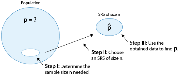
• So the fact that the expression above for determining the sample size depends on \( \hat{p} \) is problematic.




• The way to overcome this problem is to take the conservative approach by setting \( \hat{p} = 1/2 \) .




• Why do we call this approach conservative?




• It is conservative because the expression that appears in the numerator, \( 4\hat{p}(1 - \hat{p}) \) is maximized when \( \hat{p} = 1/2 \).




• That way, the n we get will work in giving us the desired margin of error regardless of what the value of \( \hat{p} \) is. This is a "worst case scenario" approach. So when we do that we get: \( n = \frac{(4)(1/2)(1 - 1/2)}{m^2} = \frac{1}{m^2} \)




• Example




1. It seems like media polls usually use a sample size of 1,000 to 1,200. This could be puzzling.




2. How could the results obtained from, say, 1,100 U.S. adults give us information about the entire population of U.S. adults? 1,100 is such a tiny fraction of the actual population. Here is the answer:




3. What sample size n is needed if a margin of error m = 0.03 is desired? \( n = \frac{1}{.03^2} = 1111.11 \rightarrow n = 1112 \) (remember, always round up). In fact, .03 is a very commonly used margin of error, especially for media polls. For this reason, most media polls work with a sample of around 1,100 people.




• Example




1. A few days before an election, a media outlet would like to estimate p, the proportion of eligible voters who support the Democratic candidate. The media outlet would like the estimate to be within 1% (that is, 0.01) of the true proportion. What is the sample size needed to achieve this in a poll?




2. Set \( n = \frac{1}{m^2} = \frac{1}{.01^2} = 10000 \).




3. Note that if we take the same conservative approach for the margin of error: \( m = 2\sqrt{\frac{\hat{p}(1-\hat{p})}{n}}\)




4. and use \( \hat{p} = 1/2 \), we'll get




5. \( m = 2\sqrt{\frac{(4)(1/2)(1-1/2)}{n}} = \frac{1}{\sqrt{n}}\),




6. a conservative estimate for the margin of error, which is useful when we want to get a rough idea of its size without taking the trouble to make detailed calculations.




7. Also, typically, there are several questions in polls, each yielding a different \( \hat{p} \).




8. Rather than reporting the separate margin of error for each question using \( m = 2\sqrt{\frac{\hat{p}(1-\hat{p})}{n}} \), polls report just one, the conservative margin of error \( m = \frac{1}{\sqrt{n}} \) as the margin of error of the poll, which is guaranteed to work for all the questions regardless what the value of \( \hat{p} \) ends up being.




• Example




1. A random sample of 2,500 U.S. adults was chosen to participate in a public opinion survey about different issues related to crime. What is the margin of error of this survey?




2. We'll simply use \( m = \frac{1}{\sqrt{n}} = \frac{1}{\sqrt{2500}} = 0.02 \) . The survey has a margin of error of 2%. This means that for each of the questions asked, the obtained sample proportion will be within 2% of the proportion among all U.S. adults.

View Answer



View Answer



View Answer

• As we did for the mean, the assumption we made in order to develop the methods in this unit was that the sampling distribution of the sample proportion, \( \hat{p} \), is roughly normal. Recall from module 4 of the Probability unit that the conditions under which this happens are that \( n * p \geq 10 \) and \( n * (1 - p) \geq 10\). Since p is unknown, we will replace it with its estimate, the sample proportion, and set




• \( n * \hat{p} \geq 10 \) and \(n * ( 1 - \hat{p} \geq 10 )\) to be the conditions under which it is safe to use the methods we developed




• Scenario: Ban on Assault Weapons




1. Background: The U.S. federal ban on assault weapons expired in September 2004, which meant that after 10 years (since the ban was instituted in 1994) there were certain types of guns that could be manufactured legally again.




2. A poll asked a random sample of 1,200 eligible voters (among other questions) whether they were satisfied with the fact that the law had expired.




3. Data are based on a poll conducted by NBC News/Wall Street Journal.




4. We would like to estimate p, the proportion of U.S. eligible voters who were satisfied with the expiration of the law, with a 95% confidence interval.




5. Based on the sample size, what is the margin of error of this poll? Report your answer as a proportion (0.000 to 1.000) rounded to THREE decimal places.

View Answer



View Answer

Q. Why is there an apparent discrepancy between the margin of error calculated using the sample size and the margin of error calculated from the 95% confidence interval?

• We found that the margin of error of this poll is roughly 2.9% using the sample size and a margin of error is 2% using the 95% confidence interval.




• This is because when we used the sample size we calculated a "conservative" margin of error. This margin of error is the margin of error *of the whole poll*.




• What it says is: Based on this sample size, the margin of error for *any* of the questions in this poll will be no more than 2.9% regardless of what the sample proportions are.




• In the particular question about the ban on assault weapons from the poll, the margin of error happened to be lower (2%).

Summarize :

1. In general, a confidence interval for the unknown population proportion (p) is \( \hat{p} \pm z* . \sqrt{ \frac{\hat{p}(1 - \hat{p})}{n} }\), where z* is 1.645 for 90% confidence, 2 for 95% confidence, and 2.576 for 99% confidence.




2. To obtain a desired margin of error (m) in a 95% confidence interval for unknown population proportion, a conservative sample size is \(n = \frac{1}{m^2}\).




3. The margin of error of a poll is determined (conservatively) by \( \frac{1}{\sqrt{n}} \).




4. The methods developed in this unit are safe to use as long as \(n * \hat{p} \geq 10 \) and \( n * (1 - \hat{p}) \geq 10 \) .

Previous

Next