• Example




• A case of suspected cheating on an exam is brought in front of the disciplinary committee at a certain university.




• There are two opposing claims in this case:




1. The student's claim: I did not cheat on the exam.




2. The instructor's claim: The student did cheat on the exam.




• Adhering to the principle "innocent until proven guilty," the committee asks the instructor for evidence to support his claim. The instructor explains that the exam had two versions, and shows the committee members that on three separate exam questions, the student used in his solution numbers that were given in the other version of the exam.




• The committee members all agree that it would be extremely unlikely to get evidence like that if the student's claim of not cheating had been true. In other words, the committee members all agree that the instructor brought forward strong enough evidence to reject the student's claim, and conclude that the student did cheat on the exam.




• Statistical hypothesis testing is defined as:




1. Assessing evidence provided by the data in favor of or against some claim about the population.




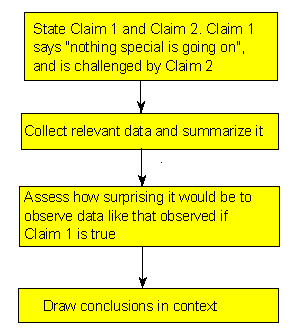
• Here is how the process of statistical hypothesis testing works:




• We have two claims about what is going on in the population. Let's call them for now claim 1 and claim 2. Much like the story above, where the student's claim is challenged by the instructor's claim, claim 1 is challenged by claim 2. (Comment: as you'll see in the examples that follow, these claims are usually about the value of population parameter(s) or about the existence or nonexistence of a relationship between two variables in the population).




• We choose a sample, collect relevant data and summarize them (this is similar to the instructor collecting evidence from the student's exam).




• We figure out how likely it is to observe data like the data we got, had claim 1 been true. (Note that the wording "how likely ..." implies that this step requires some kind of probability calculation). In the story, the committee members assessed how likely it is to observe the evidence like that which the instructor provided, had the student's claim of not cheating been true.




• Based on what we found in the previous step, we make our decision:




• If we find that if claim 1 were true it would be extremely unlikely to observe the data that we observed, then we have strong evidence against claim 1, and we reject it in favor of claim 2.




• If we find that if claim 1 were true observing the data that we observed is not very unlikely, then we do not have enough evidence against claim 1, and therefore we cannot reject it in favor of claim 2.




• In our story, the committee decided that it would be extremely unlikely to find the evidence that the instructor provided had the student's claim of not cheating been true. In other words, the members felt that it is extremely unlikely that it is just a coincidence that the student used the numbers from the other version of the exam on three separate problems. The committee members therefore decided to reject the student's claim and concluded that the student had, indeed, cheated on the exam.




• Hopefully this example helped you understand the logic behind hypothesis testing. To strengthen your understanding of the process of hypothesis testing and the logic behind it, let's look at three statistical examples.




• Example: 1




1. A recent study estimated that 20% of all college students in the United States smoke. The head of Health Services at Goodheart University suspects that the proportion of smokers may be lower there. In hopes of confirming her claim, the head of Health Services chooses a random sample of 400 Goodheart students, and finds that 70 of them are smokers.




2. Let's analyze this example using the 4 steps outlined above:




3. Stating the claims:




4. There are two claims here:




1. claim 1: The proportion of smokers at Goodheart is 0.20.




2. claim 2: The proportion of smokers at Goodheart is less than 0.20.




5. Claim 1 basically says "nothing special goes on in Goodheart University; the proportion of smokers there is no different from the proportion in the entire country." This claim is challenged by the head of Health Services, who suspects that the proportion of smokers at Goodheart is lower.




6. Choosing a sample and collecting data:




7. A sample of n = 400 was chosen, and summarizing the data revealed that the sample proportion of smokers is \( \hat{p} = \frac{70}{400} = 0.175 \).




8. While it is true that 0.175 is less than 0.20, it is not clear whether this is strong enough evidence against claim 1.




9. Assessment of evidence:




10. In order to assess whether the data provide strong enough evidence against claim 1, we need to ask ourselves: How surprising is it to get a sample proportion as low as \( \hat{p} = 0.175 \) (or lower), assuming claim 1 is true?




11. In other words, we need to find how likely it is that in a random sample of size n = 400 taken from a population where the proportion of smokers is p = 0.20 we'll get a sample proportion as low as \( \hat{p} = 0.175 \) (or lower).




12. It turns out that the probability that we'll get a sample proportion as low as \( \hat{p} = 0.175 \) (or lower) in such a sample is roughly 0.106.




13. Conclusion:




1. Well, we found that if claim 1 were true there is a probability of 0.106 of observing data like that observed.




2. Do you think that a probability of 0.106 makes our data rare enough (surprising enough) under claim 1 so that the fact that we did observe it is enough evidence to reject claim 1?




3. Or do you feel that a probability of 0.106 means that data like we observed are not very likely when claim 1 is true, but they are not unlikely enough to conclude that getting such data is sufficient evidence to reject claim 1.

• Example: 2 - A certain prescription allergy medicine is supposed to contain an average of 245 parts per million (ppm) of a certain chemical. If the concentration is higher than 245 ppm, the drug will likely cause unpleasant side effects, and if the concentration is below 245 ppm, the drug may be ineffective. The manufacturer wants to check whether the mean concentration in a large shipment is the required 245 ppm or not. To this end, a random sample of 64 portions from the large shipment is tested, and it is found that the sample mean concentration is 250 ppm with a sample standard deviation of 12 ppm. Let's analyze this example according to the four steps of hypotheses testing we outlined on the previous page:




• Stating the claims:




1. Claim 1: The mean concentration in the shipment is the required 245 ppm.




2. Claim 2: The mean concentration in the shipment is not the required 245 ppm.




• Note that again, claim 1 basically says: "There is nothing unusual about this shipment, the mean concentration is the required 245 ppm." This claim is challenged by the manufacturer, who wants to check whether that is, indeed, the case or not.




• Choosing a sample and collecting data:




1. A sample of n = 64 portions is chosen and after summarizing the data it is found that the sample concentration is and the sample standard deviation is s = 12.




2. Is the fact that is different from 245 strong enough evidence to reject claim 1 and conclude that the mean concentration in the whole shipment is not the required 245? In other words, do the data provide strong enough evidence to reject claim 1?




• Assessing the evidence:




1. In order to assess whether the data provide strong enough evidence against claim 1, we need to ask ourselves the following question: If the mean concentration in the whole shipment were really the required 245 ppm (i.e., if claim 1 were true), how surprising would it be to observe a sample of 64 portions where the sample mean concentration is off by 5 ppm or more (as we did)? It turns out that it would be extremely unlikely to get such a result if the mean concentration were really the required 245. There is only a probability of 0.0007 (i.e., 7 in 10,000) of that happening.




• Making conclusions:




1. Here, it is pretty clear that a sample like the one we observed is extremely rare (or extremely unlikely) if the mean concentration in the shipment were really the required 245 ppm. The fact that we did observe such a sample therefore provides strong evidence against claim 1, so we reject it and conclude with very little doubt that the mean concentration in the shipment is not the required 245 ppm.




• Example: 3 - Is there a relationship between gender and combined scores (Math + Verbal) on the SAT exam? Following a report on the College Board website, which showed that in 2003, males scored generally higher than females on the SAT exam (http://www.collegeboard.com/prod_downloads/about/news_info/cbsenior/yr2003/pdf/2003CBSVM.pdf), an educational researcher wanted to check whether this was also the case in her school district. The researcher chose random samples of 150 males and 150 females from her school district, collected data on their SAT performance and found the following:




• Males

  n	mean	standard deviation
  150	1025	212




• Females

  n	mean	standard deviation
  150	1010	206




• Again, let's see how the process of hypothesis testing works for this example:




• Stating the claims:




1. Claim 1: Performance on the SAT is not related to gender (males and females score the same).




2. Claim 2: Performance on the SAT is related to gender - males score higher.




• Note that again, claim 1 basically says: "There is nothing going on between the variables SAT and gender." Claim 2 represents what the researcher wants to check, or suspects might actually be the case.




• Choosing a sample and collecting data: - Data were collected and summarized as given above.




1. Is the fact that the sample mean score of males (1,025) is higher than the sample mean score of females (1,010) by 15 points strong enough information to reject claim 1 and conclude that in this researcher's school district, males score higher on the SAT than females?




• Assessment of evidence:




1. In order to assess whether the data provide strong enough evidence against claim 1, we need to ask ourselves: If SAT scores are in fact not related to gender (claim 1 is true), how likely is it to get data like the data we observed, in which the difference between the males' average and females' average score is as high as 15 points or higher? It turns out that the probability of observing such a sample result if SAT score is not related to gender is approximately 0.29




• Conclusion:




1. Here, we have an example where observing a sample like the one we observed is definitely not surprising (roughly 30% chance) if claim 1 were true (i.e., if indeed there is no difference in SAT scores between males and females). We therefore conclude that our data does not provide enough evidence for rejecting claim 1.




• Comment




1. "The data provide enough evidence to reject claim 1 and accept claim 2"; or




2. "The data do not provide enough evidence to reject claim 1."




3. In particular, note that in the second type of conclusion we did not say: "I accept claim 1," but only "I don't have enough evidence to reject claim 1." We will come back to this issue later, but this is a good place to make you aware of this subtle difference.




4. 

View Answer



View Answer



View Answer

• Hypothesis testing step 1: Stating the claims.




• In all three examples, our aim is to decide between two opposing points of view, Claim 1 and Claim 2. In hypothesis testing, Claim 1 is called the null hypothesis (denoted "H0"), and Claim 2 plays the role of the alternative hypothesis (denoted "Ha").




• As we saw in the three examples, the null hypothesis suggests nothing special is going on; in other words, there is no change from the status quo, no difference from the traditional state of affairs, no relationship.




• In contrast, the alternative hypothesis disagrees with this, stating that something is going on, or there is a change from the status quo, or there is a difference from the traditional state of affairs. The alternative hypothesis, Ha, usually represents what we want to check or what we suspect is really going on.




• Let's go back to our three examples and apply the new notation:




• In example 1:




1. H0: The proportion of smokers at Goodheart is 0.20.




2. Ha: The proportion of smokers at Goodheart is less than 0.20.




• In example 2:




1. H0: The mean concentration in the shipment is the required 245 ppm.




2. Ha: The mean concentration in the shipment is not the required 245 ppm.




• In example 3:




1. H0: Performance on the SAT is not related to gender (males and females score the same).




2. Ha: Performance on the SAT is related to gender - males score higher.

View Answer



View Answer



View Answer



View Answer



View Answer



View Answer

• Hypothesis testing step 2: Choosing a sample and collecting data.




1. You look at sampled data in order to draw conclusions about the entire population. In the case of hypothesis testing, based on the data, you draw conclusions about whether or not there is enough evidence to reject Ho.




2. In this step we collect data and summarize it. Go back and look at the second step in our three examples. Note that in order to summarize the data we used simple sample statistics such as the sample proportion \( \hat{p} \), sample mean \( \overline{x} \) and the sample standard deviation (s).




3. In practice, you go a step further and use these sample statistics to summarize the data with what's called a test statistic. We are not going to go into any details right now, but we will discuss test statistics when we go through the specific tests.




• Hypothesis testing step 3: Assessing the evidence.




1. As we saw, this is the step where we calculate how likely is it to get data like that observed when Ho true. In a sense, this is the heart of the process, since we draw our conclusions based on this probability. If this probability is very small, then that means that it would be very surprising to get data like that observed if H0 were true. The fact that we did observe such data is therefore evidence against H0, and we should reject it. On the other hand, if this probability is not very small this means that observing data like that observed is not very surprising if H0 were true, so the fact that we observed such data does not provide evidence against Ho. This crucial probability, therefore, has a special name. It is called the p-value of the test.




2. In our three examples, the p-values were given to you (and you were reassured that you didn't need to worry about how these were derived):




1. Example 1: p-value = 0.106




2. Example 2: p-value = 0.0007




3. Example 3: p-value = 0.29




3. Obviously, the smaller the p-value, the more surprising it is to get data like ours when H0 is true, and therefore, the stronger the evidence the data provide against H0. Looking at the three p-values of our three examples, we see that the data that we observed in example 2 provide the strongest evidence against the null hypothesis, followed by example 1, while the data in example 3 provides the least evidence against H0.




• Comments:




1. Right now we will not go into specific details about p-value calculations, but just mention that since the p-value is the probability of getting data like those observed when H0 is true, it would make sense that the calculation of the p-value will be based on the data summary, which, as we mentioned, is the test statistic.




2. It should be noted that in the past, before statistical software was such an integral part of intro stats courses it was common to use critical values (rather than p-values) in order to assess the evidence provided by the data.

• Since our conclusion is based on how small the p-value is, or in other words, how surprising our data are when Ho is true, it would be nice to have some kind of guideline or cutoff that will help determine how small the p-value must be, or how "rare" (unlikely) our data must be when Ho is true, for us to conclude that we have enough evidence to reject Ho.




• This cutoff exists, and because it is so important, it has a special name. It is called the significance level of the test and is usually denoted by the Greek letter α. The most commonly used significance level is α = 0.05 (or 5%). This means that:




• if the p-value < α (usually 0.05), then the data we got is considered to be "rare (or surprising) enough" when Ho is true, and we say that the data provide significant evidence against Ho, so we reject Ho and accept Ha.




• if the p-value > α (usually 0.05), then our data are not considered to be "surprising enough" when Ho is true, and we say that our data do not provide enough evidence to reject Ho (or, equivalently, that the data do not provide enough evidence to accept Ha).




• Important comment about wording - Another common wording (mostly in scientific journals) is:




1. "The results are statistically significant" - when the p-value < α.




2. "The results are not statistically significant" - when the p-value > α.




• Comments




1. Although the significance level provides a good guideline for drawing our conclusions, it should not be treated as an incontrovertible truth. There is a lot of room for personal interpretation. What if your p-value is 0.052? You might want to stick to the rules and say "0.052 > 0.05 and therefore I don't have enough evidence to reject Ho", but you might decide that 0.052 is small enough for you to believe that Ho should be rejected.




2. It should be noted that scientific journals do consider 0.05 to be the cutoff point for which any p-value below the cutoff indicates enough evidence against Ho, and any p-value above it, or even equal to it, indicates there is not enough evidence against Ho.




3. It is important to draw your conclusions in context. It is never enough to say: "p-value = ..., and therefore I have enough evidence to reject Ho at the .05 significance level."You should always add: "... and conclude that ... (what it means in the context of the problem)".




• Either I reject Ho and accept Ha (when the p-value is smaller than the significance level) or I cannot reject Ho (when the p-value is larger than the significance level).




• As we mentioned earlier, note that the second conclusion does not imply that I accept Ho, but just that I don't have enough evidence to reject it. Saying (by mistake) "I don't have enough evidence to reject Ho so I accept it" indicates that the data provide evidence that Ho is true, which is not necessarily the case. Consider the following slightly artificial yet effective example:




• Example




1. An employer claims to subscribe to an "equal opportunity" policy, not hiring men any more often than women for managerial positions. Is this credible? You're not sure, so you want to test the following two hypotheses:




1. Ho: The proportion of male managers hired is 0.5




2. Ha: The proportion of male managers hired is more than 0.5




2. Data: You choose at random three of the new managers who were hired in the last 5 years and find that all 3 are men.




3. Assessing Evidence: If the proportion of male managers hired is really 0.5 (Ho is true), then the probability that the random selection of three managers will yield three males is therefore 0.5 * 0.5 * 0.5 = 0.125. This is the p-value.




4. Conclusion: Using .05 as the significance level, you conclude that since the p-value = 0.125 > 0.05, the fact that the three randomly selected mangers were all males is not enough evidence to reject Ho. In other words, you do not have enough evidence to reject the employer's claim of subscribing to an equal opportunity policy.




5. However, the data (all three selected are males) definitely does not provide evidence to accept the employer's claim (Ho).

Scenario: Opinions on Gay Marriage

• The following two hypotheses are tested:




1. Ho: The proportion of U.S. adults who oppose gay marriage is roughly 50%.




2. Ha: The proportion of U.S. adults who oppose gay marriage is above 50% (i.e., the majority oppose).




• Suppose a survey was conducted in which a random sample of 1,100 U.S. adults was asked about their opinions about gay marriage, and based on the data, the p-value was found to be 0.002.




• Comment: Throughout this activity use a 0.05 (5%) significance level (cutoff).

View Answer



View Answer



View Answer



View Answer

Scenario: Annual Miles Driven

• The following two hypotheses are tested:




1. Ho: The average number of miles driven per year is 12,000.




2. Ha: The average number of miles driven per year is less than 12,000.




• In a survey, 1,600 randomly selected drivers were asked the number of miles they drive yearly. Based upon the results, the p-value = 0.068.




• Comment: Throughout this activity use a 0.05 (5%) significance level.

View Answer



View Answer



View Answer



View Answer

• In hypothesis testing, we have two claims about the population which we call the null hypothesis, Ho, and the alternative hypothesis, Ha.




• The alternative hypothesis challenges the null hypothesis and represents what we want to check - or what we suspect might be true.




• Our goal is to decide whether we can reject the null hypothesis and accept the alternative hypothesis or not.




• In order to do that we obtain a random sample, collect relevant data, and summarize it.




• We mentioned that the data is summarized by a test statistic but we haven't gone into any details about it yet.




• Based on the data and in particular the test statistic we find the p value of the test - the probability of observing data like that observed when the null hypothesis Ho is true.




• Finally, based on the p value we draw our conclusions. When the p value is small - in particular less than the significance level which is most commonly chosen as .05 - we conclude that the data provide significant evidence to reject the null hypothesis and accept the alternative.




• If the p value is not small, we conclude that the data does not provide enough evidence to reject the null hypothesis and so we cannot accept the alternative.




• Recall that we never conclude that we accept the null hypothesis, but just that we cannot reject it.




• This is an excellent opportunity to go back and look at the big picture of statistics since the process of hypothesis testing is a great example of it.




• We want to learn about the population so we obtain a random sample and collect data, summarize the data, and use probability to find the p value so we can draw conclusions about the population.




• In other words - decide whether we can reject the null hypothesis or not.

• Background: Based on the National Center of Health Statistics, the proportion of babies born at low birth weight (below 2,500 grams) in the United States is roughly 0.078, or 7.8% (based on all the births in the United States in the year 2002). A study was done in order to check whether smoking by pregnant women increases the risk of low birth weight. In other words, the researchers wanted to check whether the proportion of babies born at low birth weight among women who smoked during their pregnancy is higher than the proportion in the general population. The researchers followed a sample of 400 women who had smoked during their pregnancy and recorded the birth weight of the newborns. Based on the data, the p-value was found to be 0.016.




• Write down the null and alternative hypotheses (Ho and Ha) that are being tested here.






1. Ho: The proportion of low birth weight births among women who smoke during the pregnancy is 0.078 (same as in the general population).




2. Ha: The proportion of low birth weight births among women who smoke during the pregnancy is higher than 0.078.




3. Recall that as we learned, the null hypothesis (Ho) says that "nothing special is going on" or there is no change from the known proportion of 0.078. The alternative hypothesis (Ha) challenges Ho and represents what the study wanted to check.

Based on the p-value, what is your conclusion (use a 0.05 significance level)?

• The p-value of the test is 0.016, which means that it is very unlikely (probability of 0.016) that we will observe data like those observed if indeed smoking does not increase the risk of low birth weight (Ho is true). In particular, since the p-value is less than 0.05, we conclude that the data provide enough evidence to conclude that the proportion of low birth weight babies born to mothers who smoked during their pregnancy is higher than the overall proportion of low birth weight babies in the population.

• The same researchers also wanted to examine whether second-hand smoking (exposure to a another person smoking) by pregnant women increases the risk of low birth weight (i.e., the proportion of babies born at a low birth weight among women who were second-hand smokers during their pregnancy is higher than the proportion in the general population). The researchers obtained a sample of 175 pregnant women who were second-hand smokers, followed them during their pregnancies, and found that 10.2% of the newborns had low birth weight. Based on these data, the p-value was found to be 0.119.

Write down the null and alternative hypotheses (Ho and Ha) that are being tested here

• Ho: The proportion of low birth weight births among women who are second-hand smokers is 0.078 (same as in the general population).




• Ha: The proportion of low birth weight births among women who are second-hand smokers is higher than 0.078.




• Recall that as we learned, the null hypothesis (Ho) says that "nothing special is going on" or there is no change from the known proportion of 0.078. The alternative hypothesis (Ha) challenges Ho and represents what the study wanted to check.

Can we conclude that the results of this study provide evidence that second-hand smoking does not increase the risk of low birth weight?

• No. Recall that in hypothesis testing we can never conclude that we accept Ho (or that Ho is true). All we can say (in case we do not get a small p-value) is that we do not have enough evidence to reject Ho.




• In particular in this case we found that 10.2% of the 175 newborns were at low birth weight (which is higher than 7.8%, the overall proportion). While this result did not provide enough evidence to conclude that second-hand smoking increases the risk of low lightweight, it definitely does not provide evidence that it doesn't. (which is what Ho claims).

Based on the p-value, what is your conclusion (use .05 significance level)?

• The p-value of this test was found to be .119, which means that it is not extremely unlikely (roughly 12% chance) that we would get data like those observed if, indeed, second-hand smoking does not increase the risk of low birth weight (Ho is true). In particular, since the p-value is not less than .05, we conclude that the data do not provide enough evidence to conclude that second-hand smoking increases the risk of low birth weight.

• The first test we are going to learn is the test about the population proportion (p). This is test is widely known as the z-test for the population proportion (p).




• When we conduct a test about a population proportion, we are working with a categorical variable.




• Identifying the variable as categorical or quantitative is an important component of choosing an appropriate hypothesis test.

View Answer


View Answer


View Answer


View Answer

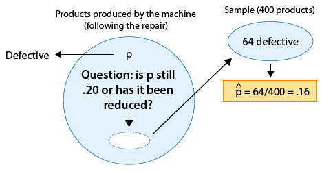
• A machine is known to produce 20% defective products, and is therefore sent for repair. After the machine is repaired, 400 products produced by the machine are chosen at random and 64 of them are found to be defective. Do the data provide enough evidence that the proportion of defective products produced by the machine (p) has been reduced as a result of the repair?




• The following figure displays the information, as well as the question of interest:




• 




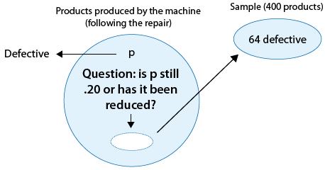
• The question of interest helps us formulate the null and alternative hypotheses in terms of p, the proportion of defective products produced by the machine following the repair:




• Ho: p = 0.20 (No change; the repair did not help).




• Ha: p < 0.20 (The repair was effective).

• There are rumors that students at a certain liberal arts college are more inclined to use drugs than U.S. college students in general. Suppose that in a simple random sample of 100 students from the college, 19 admitted to marijuana use. Do the data provide enough evidence to conclude that the proportion of marijuana users among the students in the college (p) is higher than the national proportion, which is 0.157? (This number is reported by the Harvard School of Public Health.)




• Again, the following figure displays the information as well as the question of interest:




• 




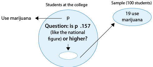
• As before, we can formulate the null and alternative hypotheses in terms of p, the proportion of students in the college who use marijuana:




• Ho: p = 0.157 (same as among all college students in the country).




• Ha: p > 0.157 (higher than the national figure).

• Polls on certain topics are conducted routinely in order to monitor changes in the public's opinions over time. One such topic is the death penalty. In 2003 a poll estimated that 64% of U.S. adults support the death penalty for a person convicted of murder. In a more recent poll, 675 out of 1,000 U.S. adults chosen at random were in favor of the death penalty for convicted murderers. Do the results of this poll provide evidence that the proportion of U.S. adults who support the death penalty for convicted murderers (p) changed between 2003 and the later poll?




• Here is a figure that displays the information, as well as the question of interest:




• 




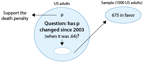
• Again, we can formulate the null and alternative hypotheses in term of p, the proportion of U.S. adults who support the death penalty for convicted murderers.




• Ho: p = 0.64 (No change from 2003).




• Ha: p ≠ 0.64 (Some change since 2003).

Scenario: Federal Grants for Community College Students

• According to the American Association of Community Colleges, 23% of community college students receive federal grants.




• The California Community College Chancellor’s Office anticipates that the percentage is smaller for California community college students.




• They collect a sample of 1,000 community college students in California and find that 210 received federal grants.

View Answer



View Answer



View Answer



View Answer



View Answer

Scenario: Number of Community College Students in the U.S.

• Using data from 2008, the American Association of Community Colleges (AACC) reports that community college students constitute 46% of all U.S. undergraduates. Given the downturn in the U.S. economy, the AACC anticipates an increase in this percentage for 2010. A poll of 500 randomly chosen undergraduates taken in 2010 indicates that 52% are attending a community college.

View Answer



View Answer

• There are basically 4 steps in the process of hypothesis testing:




1. State the null and alternative hypotheses.




2. Collect relevant data from a random sample and summarize them (using a test statistic).




3. Find the p-value, the probability of observing data like those observed assuming that Ho is true.




4. Based on the p-value, decide whether we have enough evidence to reject Ho (and accept Ha), and draw our conclusions in context.




• We are now going to go through these steps as they apply to the hypothesis testing for the population proportion p. It should be noted that even though the details will be specific to this particular test, some of the ideas that we will add apply to hypothesis testing in general.




• Stating the Hypotheses :




• Example: 1 : Has the proportion of defective products been reduced as a result of the repair?




1. Ho: p = 0.20 (No change; the repair did not help).




2. Ha: p < 0.20 (The repair was effective).




• Example: 2 - Is the proportion of marijuana users in the college higher than the national figure?




1. Ho: p = 0.157 (Same as among all college students in the country).




2. Ha: p > 0.157 (Higher than the national figure).




• Example: 3 - Did the proportion of U.S. adults who support the death penalty change between 2003 and a later poll?




1. Ho: p = 0.64 (No change from 2003).




2. Ha: p ≠ 0.64 (Some change since 2003).




• Note that the null hypothesis always takes the form:




1. Ho: p = some value




2. and the alternative hypothesis takes one of the following three forms:




3. Ha: p < that value (like in example 1) or




4. Ha: p > that value (like in example 2) or




5. Ha: p ≠ that value (like in example 3).




• Note that it was quite clear from the context which form of the alternative hypothesis would be appropriate. The value that is specified in the null hypothesis is called the null value, and is generally denoted by po. We can say, therefore, that in general the null hypothesis about the population proportion (p) would take the form: - Ho: p = po




• We write Ho: p = po to say that we are making the hypothesis that the population proportion has the value of po. In other words, p is the unknown population proportion and po is the number we think p might be for the given situation.




• The alternative hypothesis takes one of the following three forms (depending on the context):




1. Ha: p < po (one-sided)




2. Ha: p > po (one-sided)




3. Ha: p ≠ po (two-sided)




• The first two possible forms of the alternatives (where the = sign in Ho is challenged by < or >) are called one-sided alternatives, and the third form of alternative (where the = sign in Ho is challenged by ≠) is called a two-sided alternative. To understand the intuition behind these names let's go back to our examples.




• Example 3 (death penalty) is a case where we have a two-sided alternative:




1. Ho: p = 0.64 (No change from 2003).




2. Ha: p ≠ 0.64 (Some change since 2003).




• In this case, in order to reject Ho and accept Ha we will need to get a sample proportion of death penalty supporters which is very different from 0.64 in either direction, either much larger or much smaller than 0.64.




• In example 2 (marijuana use) we have a one-sided alternative:




1. Ho: p = 0.157 (Same as among all college students in the country).




2. Ha: p > 0.157 (Higher than the national figure).




3. Here, in order to reject Ho and accept Ha we will need to get a sample proportion of marijuana users which is much higher than 0.157.




4. Similarly, in example 1 (defective products), where we are testing:




5. Ho: p = 0.20 (No change; the repair did not help).




6. Ha: p < 0.20 (The repair was effective).




7. in order to reject Ho and accept Ha, we will need to get a sample proportion of defective products which is much smaller than 0.20.

Scenario: Online Credit Card Fraud

• The UCLA Internet Report (February 2003) estimated that roughly 8.7% of Internet users are extremely concerned about credit card fraud when buying online. Has that figure changed since?




• To test this, a random sample of 100 Internet users was chosen, and when interviewed, 10 said that they were extremely worried about credit card fraud when buying online.




• Let p be the proportion of all Internet users who are concerned about credit card fraud.

View Answer



View Answer

Scenario: Dial-up Internet Access

• The UCLA Internet Report (February 2003) estimated that a proportion of roughly .75 of online homes are still using dial-up access, but claimed that the use of dial-up is declining.




• Is that really the case? To examine this, a follow-up study was conducted a year later in which out of a random sample of 1,308 households that had Internet access, 804 were connecting using a dial-up modem.




• Let p be the proportion of all U.S. Internet-using households that have dial-up access.

View Answer



View Answer

• 2. Collecting and Summarizing the Data (Using a Test Statistic)




• After the hypotheses have been stated, the next step is to obtain a sample (on which the inference will be based), collect relevant data, and summarize them.




• It is extremely important that our sample is representative of the population about which we want to draw conclusions. This is ensured when the sample is chosen at random. Beyond the practical issue of ensuring representativeness, choosing a random sample has theoretical importance.




• In the case of hypothesis testing for the population proportion (p), we will collect data on the relevant categorical variable from the individuals in the sample and start by calculating the sample proportion, \( \hat{p} \) (the natural quantity to calculate when the parameter of interest is p).




1. Example: 1




2. 




3. Example: 2




4. 




5. Example: 3




6. 




• As we mentioned earlier without going into details, when we summarize the data in hypothesis testing, we go a step beyond calculating the sample statistic and summarize the data with a test statistic.




• Every test has a test statistic, which to some degree captures the essence of the test. In fact, the p-value, which so far we have looked upon as "the king" (in the sense that everything is determined by it), is actually determined by (or derived from) the test statistic.




• We will now gradually introduce the test statistic.




• The test statistic is a measure of how far the sample proportion \( \hat{p} \) is from the null value \( p_0 \), the value that the null hypothesis claims is the value of p. In other words, since \( \hat{p} \) is what the data estimates p to be, the test statistic can be viewed as a measure of the "distance" between what the data tells us about p and what the null hypothesis claims p to be.




• Example: 1 The parameter of interest is p, the proportion of defective products following the repair.




1. The data estimate p to be \( \hat{p} = 0.16 \). The null hypothesis claims that p = 0.20




2. The data are therefore 0.04 (or 4 percentage points) below the null hypothesis with respect to what they each tell us about p.




3. It is hard to evaluate whether this difference of 4% in defective products is enough evidence to say that the repair was effective, but clearly, the larger the difference, the more evidence it is against the null hypothesis. So if, for example, our sample proportion of defective products had been, say, 0.10 instead of 0.16, then I think you would all agree that cutting the proportion of defective products in half (from 20% to 10%) would be extremely strong evidence that the repair was effective.




• Example: 2 The parameter of interest is p, the proportion of students in a college who use marijuana.




1. The data estimate p to be \( \hat{p} = 0.19 \).




2. The null hypothesis claims that p = 0.157




3. The data are therefore 0.033 (or 3.3 percentage points) above the null hypothesis with respect to what they each tell us about p.




• Example: 3 The parameter of interest is p, the proportion of U.S. adults who support the death penalty for convicted murderers.




1. The data estimate p to be \( \hat{p} = 0.675 \) The null hypothesis claims that p = 0.64.




2. There is a difference of 0.035 (3.5 percentage points) between the data and the null hypothesis with respect to what they each tell us about p.




3. There is a problem with just looking at the difference between the sample proportion \( \hat{p} \) and the null value \( p_0 \).




4. In example 2 we have a difference of 3.3 percentage points between the data and the null hypothesis, which is approximately the same as the difference in example 3 of 3.5 percentage points. However, the difference in example 3 of 3.5 percentage points is based on a sample of size of 1,000 and therefore it is much more impressive than the difference of 3.3 percentage points in example 2, which was obtained from a sample of size of only 100.

View Answer



View Answer

• For the reason illustrated in the examples at the end of the previous page, the test statistic cannot simply be the difference \( \hat{p} - p_0 \), but must be some form of that formula that accounts for the sample size. In other words, we need to somehow standardize the difference \( \hat{p} - p_0 \) so that comparison between different situations will be possible. We are very close to revealing the test statistic, but before we construct it, let's be reminded of the following two facts from probability:




• 1. When we take a random sample of size n from a population with population proportion p, the possible values of the sample proportion \( \hat{p} \) (when certain conditions are met) have approximately a normal distribution with:




1. * mean: p




2. * standard deviation: \( \sqrt{\frac{p(1-p)}{n}} \)




• 2. The z-score of a normal value (a value that comes from a normal distribution) is: \( z = \frac{value - mean}{standard deviation} \)




1. and it represents how many standard deviations below or above the mean the value is.




2. We are finally ready to reveal the test statistic:




3. The test statistic for this test measures the difference between the sample proportion \( \hat{p} \) and the null value \( p_0 \) by the z-score (standardized score) of the sample proportion \( \hat{p} \), assuming that the null hypothesis is true (i.e., assuming that \( p = p_0 \)).




4. From fact 1, we know that the values of the sample proportion \( \hat{p} \) are normal, and we are given the mean and standard deviation.




5. Using fact 2, we conclude that the z-score of \( \hat{p} \) when \( p = p_0 \) is: \( z = \frac{\hat{p} - p_0}{\frac{p_0(1-p_0)}{n}} \)




6. This is the test statistic. It represents the difference between the sample proportion \( \hat{p} \) and the null value \( p_0 \), measured in standard deviations.




• 




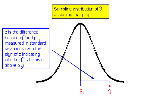
• Here is a representation of the sampling distribution of \( \hat{p} \), assuming p = po. In other words, this is a model of how \( \hat{p} \)'s behave if we are drawing random samples from a population for which Ho is true.




• Notice the center of the sampling distribution is at po, which is the hypothesized proportion given in the null hypothesis (Ho: p = po.) We could also mark the axis in standard deviation units, \( \frac{p_0(1-p_0)}{n} \) .




• For example, if our null hypothesis claims that the proportion of U.S. adults supporting the death penalty is 0.64, then the sampling distribution is drawn as if the null is true.




• We draw a normal distribution centered at p = 0.64 with a standard deviation dependent on sample size, \( \frac{0.64(1-0.64)}{n} \).




• Important Comment




• Note that under the assumption that Ho is true (i.e., \( p = p_0 \) ), the test statistic, by the nature of the fact that it is a z-score, has N(0,1) (standard normal) distribution. Another way to say the same thing which is quite common is: "The null distribution of the test statistic is N(0,1)." By "null distribution," we mean the distribution under the assumption that Ho is true. As we'll see and stress again later, the null distribution of the test statistic is what the calculation of the p-value is based on.




• Example: 1




1. 




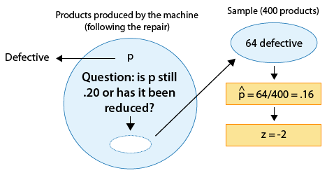
2. Since the null hypothesis is Ho: p = 0.20, the standardized score of \( \hat{p} = 0.16 \) is: \( z = \frac{0.16 - 0.2}{\sqrt{\frac{0.2(1-0.2)}{400}}} = -2 \) .




3. This is the value of the test statistic for this example.




4. This z-score of -2 tells me that (assuming that Ho is true) the sample proportion \( \hat{p} = 0.16 \) is 2 standard deviations below the null value (0.20).




• Example: 2




1. 




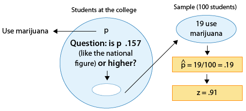
2. Since the null hypothesis is Ho: p = 0.157, the standardized score of \( \hat{p} = 0.19 \) is: \( z = \frac{0.19 - 0.157}{\sqrt{\frac{0.157(1-0.157)}{100}}} \sim 0.91 \).




3. This is the value of the test statistic for this example.




4. We interpret this to mean that, assuming that Ho is true, the sample proportion \( \hat{p} = 0.19 \) is 0.91 standard deviations above the null value (0.157).




• Example: 3




1. 




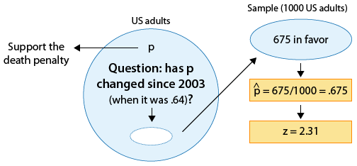
2. Since the null hypothesis is Ho: p = 0.64, the standardized score of \( \hat{p} = 0.675 \) is: \( z = \frac{0.675 - 0.64}{\sqrt{\frac{0.64(1-0.64)}{1000}}} \sim 2.31 \).




3. This is the value of the test statistic for this example.




4. We interpret this to mean that, assuming that Ho is true, the sample proportion \( \hat{p} = 0.675 \) is 2.31 standard deviations above the null value (0.64).

Comments About the Test Statistic

• We mentioned earlier that to some degree, the test statistic captures the essence of the test. In this case, the test statistic measures the difference between \( \hat{p} \) and \( p_0 \) in standard deviations.




• This is exactly what this test is about. Get data, and look at the discrepancy between what the data estimates p to be (represented by \( \hat{p} \)) and what Ho claims about p (represented by \( p_0 \) ).




• You can think about this test statistic as a measure of evidence in the data against Ho. The larger the test statistic, the "further the data are from Ho" and therefore the more evidence the data provide against Ho.

View Answer



View Answer



View Answer



View Answer



View Answer



View Answer



View Answer



View Answer



View Answer



View Answer



View Answer



View Answer



View Answer

Previous

Next