It should now be clear why this test is commonly known as the z-test for the population proportion. The name comes from the fact that it is based on a test statistic that is a z-score.

When we take a random sample of size n from a population with population proportion p, the possible values of the sample proportion \( \hat{p} \) (when certain conditions are met) have approximately a normal distribution with a mean of ... and a standard deviation of ....

This result provides the theoretical justification for constructing the test statistic the way we did, and therefore the assumptions under which this result holds (in bold, above) are the conditions that our data need to satisfy so that we can use this test. These two conditions are:

The sample has to be random.

The conditions under which the sampling distribution of \( \hat{p} \) is normal are met. In other words:

\( n × p_0 ≥ 10 and n × (1 - p_0) ≥ 10 \)

Here we will pause to say more about condition (i.) above, the need for a random sample.

In the Probability Unit we discussed sampling plans based on probability (such as a simple random sample, cluster, or stratified sampling) that produce a non-biased sample, which can be safely used in order to make inferences about a population.

We noted in the Probability Unit that, in practice, other (non-random) sampling techniques are sometimes used when random sampling is not feasible. It is important though, when these techniques are used, to be aware of the type of bias that they introduce, and thus the limitations of the conclusions that can be drawn from them.

For our purpose here, we will focus on one such practice, the situation in which a sample is not really chosen randomly, but in the context of the categorical variable that is being studied, the sample is regarded as random.

For example, say that you are interested in the proportion of students at a certain college who suffer from seasonal allergies. For that purpose, the students in a large engineering class could be considered as a random sample, since there is nothing about being in an engineering class that makes you more or less likely to suffer from seasonal allergies.

Technically, the engineering class is a convenience sample, but it is treated as a random sample in the context of this categorical variable. On the other hand, if you are interested in the proportion of students in the college who have math anxiety, then the class of engineering students clearly could not be viewed as a random sample, since engineering students probably have a much lower incidence of math anxiety than the college population overall

n = 400, , and therefore:

\( * n × p_0 = 80 ≥ 10 * n × (1 - p_0) = 320 ≥ 10 \)

n = 100, , and therefore:

\( * n × p_0 = 15.7 ≥ 10 * n × (1 - p_0) = 84.3 ≥ 10 \)

n = 1,000, . 64 , and therefore:

\( * n × p_0 = 640 ≥ 10 * n × (1 - p_0) = 360 ≥ 10 \)

State the appropriate null and alternative hypotheses, Ho and Ha.

Obtain a random sample, collect relevant data, and check whether the data meet the conditions under which the test can be used.

If the conditions are met, summarize the data using a test statistic.

Find the p-value of the test.

Based on the p-value, decide whether or not the results are significant and draw your conclusions in context.

Intuitively, the p-value is the probability of observing data like those observed assuming that Hois true. Let's be a bit more formal:

Since this is a probability question about the data, it makes sense that the calculation will involve the data summary, the test statistic.

What do we mean by "like" those observed? By "like" we mean "as extreme or even more extreme."

Putting it all together, we get that in general:

The p-value is the probability of observing a test statistic as extreme as that observed (or even more extreme) assuming that the null hypothesis is true.

By "extreme" we mean extreme in the direction of the alternative hypothesis.

Specifically, for the z-test for the population proportion:

If the alternative hypothesis is \(H_a : p < p_0 \) (less than), then "extreme" means small, and the p-value is:

The probability of observing a test statistic as small as that observed or smaller if the null hypothesis is true.

If the alternative hypothesis is \(H_a : p > p_0 \ (greater than), then "extreme" means large, and the p-value is:

The probability of observing a test statistic as large as that observed or larger if the null hypothesis is true.

if the alternative is \(H_a : p \neq p_0 \ (different from), then "extreme" means extreme in either direction either small or large (i.e., large in magnitude), and the p-value therefore is:

The probability of observing a test statistic as large in magnitude as that observed or larger if the null hypothesis is true.

Recall the important comment from our discussion about our test statistic, \( z = \frac{\hat{p} - p_0}{\sqrt{\frac{p_0(1 - p_0)}{n}}} \)

which said that when the null hypothesis is true (i.e., when ), the possible values of our test statistic (because it is a z-score) follow a standard normal (N(0,1), denoted by Z) distribution. Therefore, the p-value calculations (which assume that Ho is true) are simply standard normal distribution calculations for the 3 possible alternative hypotheses.

The probability of observing a test statistic as small as that observed or smaller, assuming that the values of the test statistic follow a standard normal distribution. We will now represent this probability in symbols and also using the normal distribution.

\( Ha: p < p_0 ⇒ p-value = P(Z ≤ z) \)

Looking at the shaded region, you can see why this is often referred to as a left-tailed test. We shaded to the left of the test statistic, since less than is to the left.

The probability of observing a test statistic as large as that observed or larger, assuming that the values of the test statistic follow a standard normal distribution. Again, we will represent this probability in symbols and using the normal distribution.

\( Ha: p > p_0 ⇒ p-value = P(Z ≥ z) \)

Looking at the shaded region, you can see why this is often referred to as a right-tailed test. We shaded to the right of the test statistic, since greater than is to the right.

The probability of observing a test statistic which is as large as in magnitude as that observed or larger, assuming that the values of the test statistic follow a standard normal distribution.

\( Ha: p ≠ p_0 ⇒ p-value = P(Z < |z|) + P(Z ≥ |z|) = 2P(Z ≥ |z|) \)

This is often referred to as a two-tailed test, since we shaded in both directions.

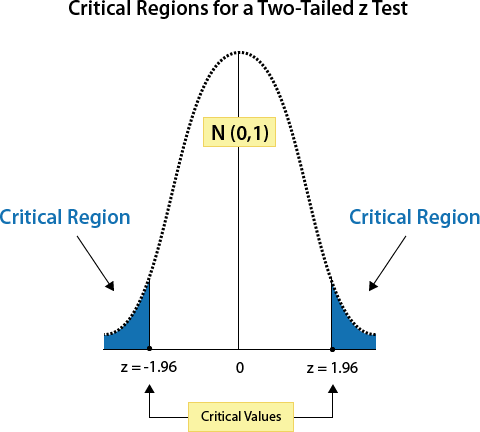
There are several concepts that are important to understand in the critical value method. They are the: 1) critical value and 2) the critical region. As shown in the graph below, the critical value is the value, which cuts off an area referred to as the critical region (or area of rejection), as applied to the z test.

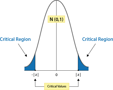
When z test statistics fall in the critical region (the blue shaded areas in the above graph), they are far enough from the mean that they are significantly different from the mean; therefore, in these instances, the null hypothesis would be rejected. The critical region is determined by a critical value that is based on two things: 1) the significance level of the test (either 0.05 or 0.01) AND the direction of the test (ex. left-tailed, right-tailed, or two-tailed).

For a two-tailed z test, there will be critical regions on both sides of the distribution. For a two-tailed test using a 0.05 level of significance, we need to determine a value that would put 0.025 or 2.5%, in each tail. We can determine this value by using the Normal Table.

First, we need to look in the body of the normal table (click here), where we will see that the exact value 0.0250 is associated with the z score of -1.96; thus, -1.96 is the critical value that puts 0.025 (or 2.5%) in the left tail of the distribution. Since the standard normal distribution is symmetrical, +1.96 is the critical value that puts 0.025 (or 2.5%) in the right tail. Thus, the critical values of -1.96 and +1.96 would define the critical regions for a two-tailed z-test using a 0.05 significance level.

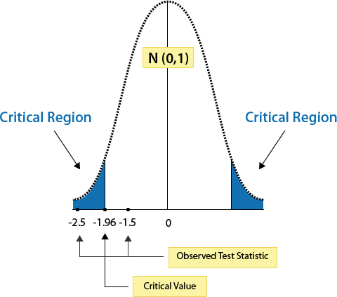
In order to test the null hypothesis, we need to look at where the z-test statistic falls in relation to the critical regions formed by the critical values. In a two-tailed z-test, a z-test statistic of -1.5 would not fall in a critical region Therefore, we know that the p-value would be more than 0.05. Thus, we would not reject the null hypothesis, since the p-value is greater than 0.05 (or, stated another way, p-value > 0.05).

On the other hand, a z-test statistic of -2.5 would fall within the critical region on the left hand side of the distribution; therefore, we know that the p-value would be less than 0.05. In this instance, we would reject the null hypothesis at a less than 0.05 level (or p-value < 0.05). Furthermore, it is possible to figure out the exact p-value for the z-test statistic of -2.5, by using the Normal Table, which is 0.0062.

The same logic applies to one-tailed z-tests. For the one-tailed “less than” z-test, the critical value for a 0.05 significance level is -1.645 (note: since the p-value for -1.64 is 0.0505 and the p-value for -1.65 is 0.0495, the critical value for 0.0500 would be between the two z scores or -1.645).

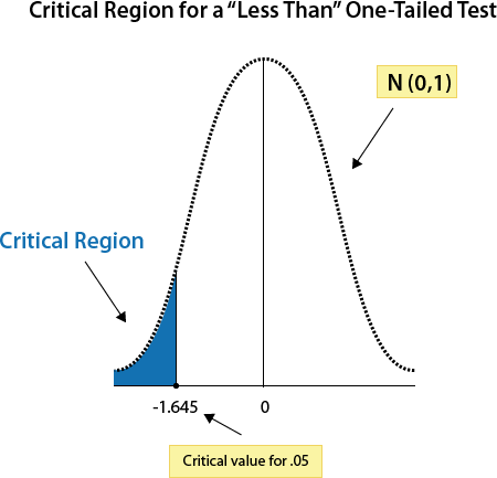
With a “less than” one-tailed z test, any z-test statistic that is less than -1.645, would fall in the critical region and therefore, would have a p-value less than 0.05. For instance, -2.5 would be less than -1.645 and would fall in the critical region. Thus, it would have a p-value less than 0.05 and the null hypothesis would be rejected.

Any z-test statistic that is larger than -1.645 would have a probability level of greater than 0.05 (or p-value > 0.05). For instance, -1.5 would be greater than -1.645 and, therefore, would not fall in the critical region. Thus, it would have a p-value greater than 0.05 and the null hypothesis would not be rejected.

For the one-tailed “greater than” z-test, the critical value for a 0.05 significance level is 1.645.

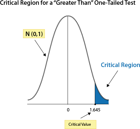
Thus, with a “greater than” one-tailed z test, any z-test statistic larger than 1.645, would fall in the critical region and therefore, would have a p-value less than 0.05. For instance, 2.5 would be greater than 1.645 and would fall in the critical region. Thus, it would have a p-value less than 0.05 (or p-value < 0.05) and the null hypothesis would be rejected .

Any z-test statistic that less than 1.645 would have a probability level of greater than 0.05 (or p-value > 0.05). For instance, 1.5 would be less than 1.645 and, therefore, would not fall in the critical region. Thus, it would have a p-value greater than 0.05 and the null hypothesis would not be rejected.

The critical value method uses two concepts: 1) the critical value and 2) the critical region. The critical value is used to determine the critical region and is based on two things: 1) the significance level of the test (either 0.05 or 0.01) AND the direction of the test (ex, left-tailed, right-tailed, or two-tailed).

When z-test statistic falls in the critical region, it is far enough from the mean that it is significantly different from the mean. Therefore, in this instance, the null hypothesis would be rejected at the significance level used to determine the critical region (either 0.05 or 0.01). Furthermore, the actual p-value can be determined by using the Normal Table.

When the z-test statistic does not fall in the critical region, it indicates that it is not far enough from the mean to be significantly different from the mean. In this instance, the null hypothesis would not be rejected.

The critical value method has been traditionally used for hypothesis testing (note: there are different critical values and tables for t-tests, ANOVAs, and Chi Square tests). The emphasis now, however, is on the use of exact p-values, which are obtained through the use of statistical software packages.

The p-value in this case is:

* The probability of observing a test statistic as small as -2 or smaller, assuming that Ho is true.

OR (recalling what the test statistic actually means in this case),

* The probability of observing a sample proportion that is 2 standard deviations or more below \(p_0 = 0.2\) , assuming that \( p_0 \) is the true population proportion.

OR, more specifically,

* The probability of observing a sample proportion of 9.16 or lower in a random sample of size 400, when the true population proportion is \(p_0 = 0.2\).

In either case, the p-value is found as shown in the following figure:

To find P(Z ≤ -2) we can either use a table or software. Eventually, after we understand the details, we will use software to run the test for us and the output will give us all the information we need. The p-value that the statistical software provides for this specific example is 0.023. The p-value tells me that it is pretty unlikely (probability of 0.023) to get data like those observed (test statistic of -2 or less) assuming that Ho is true.

The p-value in this case is:

* The probability of observing a test statistic as large as 0.91 or larger, assuming that Ho is true.

OR (recalling what the test statistic actually means in this case),

* The probability of observing a sample proportion that is 0.91 standard deviations or more above \(p_0 = 0.157\), assuming that \(p_0 \) is the true population proportion.

OR, more specifically,

* The probability of observing a sample proportion of 0.19 or higher in a random sample of size 100, when the true population proportion is \(p_0 = 0.157\).

In either case, the p-value is found as shown in the following figure:

Again, at this point we can either use a table or software to find that the p-value is 0.182.

The p-value tells us that it is not very surprising (probability of 0.182) to get data like those observed (which yield a test statistic of 0.91 or higher) assuming that the null hypothesis is true.

The p-value in this case is:

* The probability of observing a test statistic as large as 2.31 (or larger) or as small as -2.31 (or smaller), assuming that Ho is true.

OR (recalling what the test statistic actually means in this case),

* The probability of observing a sample proportion that is 2.31 standard deviations or more away from \(p_0 = 0.64\), assuming that \(p_0 \) is the true population proportion.

OR, more specifically,

* The probability of observing a sample proportion as different as 0.675 is from 0.64, or even more different (i.e. as high as 0.675 or higher or as low as 0.605 or lower) in a random sample of size 1,000, when the true population proportion is \(p_0 = 0.64\).

In either case, the p-value is found as shown in the following figure:

Again, at this point we can either use a table or software to find that the p-value is 0.021.

The p-value tells us that it is pretty unlikely (probability of 0.021) to get data like those observed (test statistic as high as 2.31 or higher or as low as -2.31 or lower) assuming that Ho is true.

We've just seen that finding p-values involves probability calculations about the value of the test statistic assuming that Ho is true. In this case, when Ho is true, the values of the test statistic follow a standard normal distribution (i.e., the sampling distribution of the test statistic when the null hypothesis is true is N(0,1)). Therefore, p-values correspond to areas (probabilities) under the standard normal curve.

Similarly, in any test, p-values are found using the sampling distribution of the test statistic when the null hypothesis is true (also known as the "null distribution" of the test statistic). In this case, it was relatively easy to argue that the null distribution of our test statistic is N(0,1).

We've just completed our discussion about the p-value, and how it is calculated both in general and more specifically for the z-test for the population proportion.

State the appropriate null and alternative hypotheses, Ho and Ha.

Obtain a random sample, collect relevant data, and check whether the data meet the conditions under which the test can be used. If the conditions are met, summarize the data using a test statistic.

Find the p-value of the test.

Based on the p-value, decide whether or not the results are significant, and draw your conclusions in context.

(i) Based on the p-value, determine whether or not the results are significant (i.e., the data present enough evidence to reject Ho).

(ii) State your conclusions in the context of the problem.

(Has the proportion of defective products been reduced from 0.20 as a result of the repair?)

We found that the p-value for this test was 0.023.

Since 0.023 is small (in particular, 0.023 < 0.05), the data provide enough evidence to reject Ho and conclude that as a result of the repair the proportion of defective products has been reduced to below 0.20. The following figure is the complete story of this example, and includes all the steps we went through, starting from stating the hypotheses and ending with our conclusions:

(Is the proportion of students who use marijuana at the college higher than the national proportion, which is 0.157?)

We found that the p-value for this test was 0.182.

Since 0.182 is not small (in particular, 0.182 > 0.05), the data do not provide enough evidence to reject Ho.

We therefore do not have enough evidence to conclude that the proportion of students at the college who use marijuana is higher than the national figure. Here is the complete story of this example:

(Has the proportion of U.S. adults who support the death penalty for convicted murderers changed since 2003, when it was 0.64?)

We found that the p-value for this test was 0.021.

Since 0.021 is small (in particular, 0.021 < 0.05), the data provide enough evidence to reject Ho, and we conclude that the proportion of adults who support the death penalty for convicted murderers has changed since 2003. Here is the complete story of this example:

Answer: This is largely due to just convenience and tradition.

When Ronald Fisher (one of the founders of modern statistics) published one of his tables, he used a mathematically convenient scale that included 5% and 1%.

Later, these same 5% and 1% levels were used by other people, in part just because Fisher was so highly esteemed. But mostly these are arbitrary levels.

The idea of selecting some sort of relatively small cutoff was historically important in the development of statistics; but it’s important to remember that there is really a continuous range of increasing confidence towards the alternative hypothesis, not a single all-or-nothing value.

There isn’t much meaningful difference, for instance, between a p-value of 0.049 or 0.051, and it would be foolish to declare one case definitely a "real" effect and to declare the other case definitely a "random" effect.

In either case, the study results were roughly 5% likely by chance if there’s no actual effect.

Whether such a p-value is sufficient for us to reject a particular null hypothesis ultimately depends on the risk of making the wrong decision, and the extent to which the hypothesized effect might contradict our prior experience or previous studies.

State the null and alternative hypotheses: \(H_0 : p = p_0 \)

\( H_a : p <, >, or ≠ p_0 \)

where the choice of the appropriate alternative (out of the three) is usually quite clear from the context of the problem.

Obtain data from a sample and:

(i) Check whether the data satisfy the conditions which allow you to use this test.

Random sample (or at least a sample that can be considered random in context) n ⋅ p0 ≥ 10, n ⋅ (1 − p0) ≥ 10

(ii) Calculate the sample proportion \( \hat{p} \), and summarize the data using the test statistic:

\( z = \frac{\hat{p} - p_0}{\sqrt{\frac{p_0(1 - p_0)}{n}}} \).

(Recall: This standardized test statistic represents how many standard deviations above or below \( p_0 \) our sample proportion \( \hat{p} \) is. )

Find the p-value of the test either by using software or by using the test statistic as follows:

* for \(H_a : p < p_0: P(Z \leq z)\)
* for \(H_a : p > p_0: P(Z \geq z)\)
* for \(H_a : p \neq p_0: 2P(Z \leq |z|)\)

Reach a conclusion first regarding the significance of the results, and then determine what it means in the context of the problem. Recall that:

If the p-value is small (in particular, smaller than the significance level, which is usually 0.05), the results are significant (in the sense that there is a significant difference between what was observed in the sample and what was claimed in Ho), and so we reject Ho. If the p-value is not small, we do not have enough statistical evidence to reject Ho, and so we continue to believe that Ho may be true. (Remember, in hypothesis testing we never "accept" Ho).