The issues regarding hypothesis testing that we will discuss are:

The effect of sample size on hypothesis testing.

Statistical significance vs. practical importance. (This will be discussed in the activity following number 1.)

One-sided alternative vs. two-sided alternative—understanding what is going on.

Hypothesis testing and confidence intervals—how are they related?

The Effect of Sample Size on Hypothesis Testing

We have already seen the effect that the sample size has on inference, when we discussed point and interval estimation for the population mean (μ) and population proportion (p).

Larger sample sizes give us more information to pin down the true nature of the population. We can therefore expect the sample mean and sample proportion obtained from a larger sample to be closer to the population mean and proportion, respectively. As a result, for the same level of confidence, we can report a smaller margin of error, and get a narrower confidence interval. What we've seen, then, is that larger sample size gives a boost to how much we trust our sample results. In hypothesis testing, larger sample sizes have a similar effect. The following two examples will illustrate that a larger sample size provides more convincing evidence, and how the evidence manifests itself in hypothesis testing.

Example: 2

The data do not provide enough evidence that the proportion of marijuana users at the college is higher than the proportion among all U.S. college students, which is 0.157. So far, nothing new. Let's make small changes to the problem (and call it example 2*). The changes are highlighted and the problem is followed by a new figure that reflects the changes.

Example: 2*

There are rumors that students in a certain liberal arts college are more inclined to use drugs than U.S. college students in general. Suppose that in a simple random sample of 400 students from the college, 76 admitted to marijuana use. Do the data provide enough evidence to conclude that the proportion of marijuana users among the students in the college (p) is higher than the national proportion, which is 0.157? (reported by the Harvard School of Public Health).

We now have a larger sample (400 instead of 100), and also we changed the number of marijuana users (76 instead of 19).

I. The question of interest did not change, so we are testing the same hypotheses:

Ho: p = 0.157

Ha: p > 0.157

II. We select a random sample of size 400 and find that 76 are marijuana users.

\( \hat{p} = \frac{76}{400} = 0.19 \)

This is the same sample proportion as in the original problem, so it seems that the data give us the same evidence, but when we calculate the test statistic, we see that actually this is not the case:

\( *z = \frac{0.19 - 0.157}{\sqrt{\frac{0.157(1 - 0.157)}{400}}} \sim 1.81 \)

Even though the sample proportion is the same (0.19), since here it is based on a larger sample (400 instead of 100), it is 1.81 standard deviations above the null value of 0.157 (as opposed to 0.91 standard deviations in the original problem).

III. For the p-value, we use statistical software to find p-value = 0.035.

The p-value here is 0.035 (as opposed to 0.182 in the original problem). In other words, when Ho is true (i.e. when p = 0.157) it is quite unlikely (probability of 0.035) to get a sample proportion of 0.19 or higher based on a sample of size 400 (probability 0.035), and not very unlikely when the sample size is 100 (probability 0.182).

IV. Our results here are significant. In other words, in example 2* the data provide enough evidence to reject Ho and conclude that the proportion of marijuana users at the college is higher than among all U.S. students.

What do we learn from these two examples?

We see that sample results that are based on a larger sample carry more weight.

In example 2, we saw that a sample proportion of 0.19 based on a sample of size of 100 was not enough evidence that the proportion of marijuana users in the college is higher than 0.157. Recall, from our general overview of hypothesis testing, that this conclusion (not having enough evidence to reject the null hypothesis) doesn't mean the null hypothesis is necessarily true (so, we never “accept” the null); it only means that the particular study didn’t yield sufficient evidence to reject the null. It might be that the sample size was simply too small to detect a statistically significant difference.

However, in example 2*, we saw that when the sample proportion of 0.19 is obtained from a sample of size 400, it carries much more weight, and in particular, provides enough evidence that the proportion of marijuana users in the college is higher than 0.157 (the national figure). In this case, the sample size of 400 was large enough to detect a statistically significant difference.

Scenario: Support of U.S. Administration's Policies Suppose that only 40% of the U.S. public supported the general direction of the previous U.S. administration's policies. To gauge whether the nationwide proportion, p, of support for the current administration is higher than 40%, a major polling organization conducts a random poll to test the hypotheses:

Ho: p = 0.40

Ha: p > 0.40

The results are reported to be not statistically significant, with a p-value of 0.214.

Suppose that only 40% of the U.S. public supported the general direction of the previous U.S. administration's policies. To gauge whether the nationwide proportion, p, of support for the current administration is higher than 40%, a major polling organization conducts a random poll to test the hypotheses: Ho: p = 0.40 Ha: p > 0.40 The results are reported to be not statistically significant, with a p-value of 0.214. Based on the study, is the following statement is a valid conclusion or an invalid conclusion? The results do not reject the null hypothesis:

valid

invalid

Explanation :

When the results are "not statistically significant," it means we don’t have sufficient evidence to reject the null hypothesis, because any difference in the study was probably just by chance. In fact, the p-value is the probability of that chance difference, and a p-value of 0.214 is considerably larger than the traditional 0.05 level below which we would begin to reject the null hypothesis

Based on the study, is the following statement is a valid conclusion or an invalid conclusion? The results provide enough evidence to accept the null hypothesis:

valid

invalid

Explanation :

We never "accept" the null hypothesis. In the case of the study described, the lack of statistical significance means there wasn’t sufficiently surprising evidence against the null, so the null hypothesis should merely remain the default conclusion until more evidence is gathered.

Based on the study, is the following statement is a valid conclusion or an invalid conclusion? The results indicate that it must be true that the nationwide proportion, p, of support for the current administration is equal to 40%:

valid

invalid

Explanation :

We never "prove" the null hypothesis. In the case of the study described, the lack of statistical significance in the study indicates we don’t have sufficient evidence to reject the null hypothesis, but that doesn’t mean the null is true; the alternative hypothesis might actually be true, and it might simply be that the study wasn’t sensitive enough to detect a real difference.

Based on the study, is the following statement is a valid conclusion or an invalid conclusion? The results indicate that the nationwide proportion, p, of support for the current administration might be greater than 40%, but the sample size in the study might have been too small to detect a statistically significant difference:

valid

invalid

Explanation :

Even though the null hypothesis can’t be rejected by this study, the alternative hypothesis might actually be true; the study might simply not have been sensitive enough to detect the difference.

Scenario: Repairs to Eliminate Defective Products The purpose of this activity is to give you guided practice exploring the effect of sample size on the significance of sample results, and help you get a better sense of this effect. Another important goal of this activity is to help you understand the distinction between statistical significance and practical importance.

The results of this study—64 defective products out of 400—were statistically significant in the sense that they provided enough evidence to conclude that the repair indeed reduced the proportion of defective products from 0.20 (the proportion prior to the repair).

Even though the results—a sample proportion of defective products of 0.16—are statistically significant, it is not clear whether the results indicate that the repair was effective enough to meet the company's needs, or, in other words, whether these results have a practical importance.

If the company expected the repair to eliminate defective products almost entirely, then even though statistically, the results indicate a significant reduction in the proportion of defective products, this reduction has very little practical importance, because the repair was not effective in achieving what it was supposed to.

To make sure you understand this important distinction between statistical significance and practical importance, we will push this a bit further.

Consider the same example, but suppose that when the company examined the 400 randomly selected products, they found that 78 of them were defective (instead of 64 in the original problem):

Note that the sample proportion of defective products is 0.195. Regardless of whether the results are statistically significant or not, comment on the practical implication of the results.

Answer: A sample proportion of 0.195 (19.5% defective products) tells us that practically, the repair was ineffective in reducing the proportion of defective products. It is hard to imagine a situation where a company would consider a reduction of 0.5% a practically important reduction in the proportion of defective products.

We conduct a z-test and get the following output:
H0: p = 0.2
HA: p < 0.2
z = -0.25, p-value = 0.4013
Based on the output, comment on the (statistical) significance of the results, and state your conclusions in context.

Answer: Based on the large p-value (0.401) we conclude that the results are not statistically significant. In other words, the data do not provide evidence to conclude that the proportion of defective products has been reduced.

Consider now another variation on the same problem. Assume now that over a period of a month following the repair, the company randomly selected 20,000 products, and found that 3,900 of them were defective.

Note that the sample proportion of defective products is the same as before, 0.195, which as we established before, does not indicate any practically important reduction in the proportion of defective products.
We conduct a z-test on the additional data and get the following output:

H0: p = 0.2
HA: p < 0.2
z = -1.76, p-value = 0.0385
Based on the output, comment on the (statistical) significance of the results and state your conclusions in context.

Answer: Even though the sample results are similar to what we got before (sample proportion of 0.195), since they are based on a much larger sample (20,000 compared to 400) now they are statistically significant (at the 0.05 level, since 0.039 is less than 0.05). In this case, we can therefore reject H0 and conclude that the repair reduced the proportion of defective products below 0.20.

Summary: This is perhaps an “extreme” example, yet it is effective in illustrating the important distinction between practical importance and statistical significance. A reduction of 0.005 (or 0.5%) in the proportion of defective products probably does not carry any practical importance, however, because of the large sample size, this reduction is statistically significant. In general, with a sufficiently large sample size you can make any result that has very little practical importance statistically significant. This suggests that when interpreting the results of a test, you should always think not only about the statistical significance of the results but also about their practical importance.

3. One-Sided Alternative vs. Two-Sided Alternative

Recall that earlier we noticed (only visually) that for a given value of the test statistic z, the p-value of the two-sided test is twice as large as the p-value of the one-sided test. We will now further discuss this issue. In particular, we will use our example 2 (marijuana users at a certain college) to gain better intuition about this fact.

For illustration purposes, we are actually going to use example 2* (where out of a sample of size 400, 76 were marijuana users). Let's recall example 2*, but this time give two versions of it; the original version, and a slightly changed version, which we'll call example 2**. The differences are highlighted.

Example: 2*

There are rumors that students at a certain liberal arts college are more inclined to use drugs than U.S. college students in general. Suppose that in a simple random sample of 400 students from the college, 76 admitted to marijuana use. Do the data provide enough evidence to conclude that the proportion of marijuana users among the students in the college (p) is higher than the national proportion, which is .157? (This number is reported by the Harvard School of Public Health.)

Example: 2**

The dean of students in a certain liberal arts college was interested in whether the proportion of students who use drugs in her college is different than the proportion among U.S. college students in general. Suppose that in a simple random sample of 400 students from the college, 76 admitted to marijuana use. Do the data provide enough evidence to conclude that the proportion of marijuana users among the students in the college (p) differs from the national proportion, which is 0.157? (This number is reported by the Harvard School of Public Health.)

Example: 2*

We already carried out the test for this example, and the results are summarized in the following figure

The following figure reminds you how the p-value was found (using the test statistic):

Example: 2**

I. Here we are testing:

\( H_0: p = 1.57 \)

\( H_a: p \neq 1.57 \)

II. Since we have the same data as in example 2* (76 marijuana users out of 400), we have the same sample proportion and the same test statistic:

\( \hat{p} = .19 \)

\( z = 1.81 \)

III. Since the calculation of the p-value depends on the type of alternative we have, here is where things start to be different. Statistical software tells us that the p-value for example 2** is 0.070. Here is a figure that reminds us how the p-value was calculated (based on the test statistic):

IV. If we use the 0.05 level of significance, the p-value we got is not small enough (0.07 > 0.05), and therefore we cannot reject Ho. In other words, the data do not provide enough evidence to conclude that the proportion of marijuana smokers in the college is different from the national proportion (0.157).

It should be pretty clear what happened here numerically. The p-value of the one-sided test (example 2*) is 0.035, suggesting the results are significant at the 0.05 significant level. However, the p-value of the two sided-test (example 2**) is twice the p-value of the one-sided test, and is therefore 2 * 0.035 = 0.07, suggesting that the results are not significant at the 0.05 significance level.

The idea is that in Example 2*, we began our hypothesis test with a piece of information (in the form of a rumor) about unknown population proportion p, which gave us a sort of head-start towards the goal of rejecting the null hypothesis. We found that the evidence that the data provided were then enough to cross the finish line and reject Ho. In Example 2**, we had no prior information to go on, and the data alone were not enough evidence to cross the finish line and reject Ho. The following figure illustrates this idea

We can summarize and say that in general it is harder to reject Ho against a two-sided Ha because the p-value is twice as large. Intuitively, a one-sided alternative gives us a head-start, and on top of that we have the evidence provided by the data. When our alternative is the two-sided test, we get no head-start and all we have are the data, and therefore it is harder to cross the finish line and reject Ho.

Read the two versions carefully. In particular, pay attention to the highlighted parts. What is the main difference between the two versions?

In example 2** we are told that the dean of students initiated the study, and in example 2* we don't know who did.

In example 2* the alternative is one-sided (Ho: p > 0.157), and the new wording in example 2** suggests that the two-sided alternative is appropriate.

Explanation :

Indeed, in example 2* we suspect from the outset (based on the rumors) that the overall proportion (p) of marijuana smokers at the college is higher than the reported national proportion of 0.157, and therefore the appropriate alternative is Ho: p > 0.157. Indeed, in example 2* we suspect from the outset (based on the rumors) that the overall proportion (p) of marijuana smokers at the college is higher than the reported national proportion of 0.157, and therefore the appropriate alternative is Ho: p > 0.157. In example 2**, as a result of the change of wording (which eliminated the part about the rumors), we simply wonder if p is different (in either direction) from the reported national proportion of 0.157, and therefore the appropriate alternative is the two-sided test: \( H_a : p \neq p_0 \). Would switching to the two-sided alternative have an effect on our results?

Consider the following two hypothesis testing scenarios for the population proportion (p) and corresponding studies: I. The UCLA Internet Report (February 2003) estimated that roughly 8.7% of Internet users are extremely concerned about credit card fraud when buying online. A study was designed in order to examine whether that proportion has changed since. II. The UCLA Internet Report (February 2003) estimated that roughly 8.7% of Internet users are extremely concerned about credit card fraud when buying online. In light of the increasing problem of spyware, a study was designed in order to examine whether that proportion has increased since. Assume that the two studies (I and II) used the same data, and that the p-value of the test corresponding to study I was found to be 0.024. The p-value of the test corresponding to study II:

must be 0.012

must be 0.048.

Explanation :

Indeed, in study I we are testing Ho: p = 0.087 and Ha: p ≠ 0.087, whereas in study II, we are testing: Ho: p = 0.087 and Ha: p > 0.087. Since the p-value of the two-sided test is always twice the p-value of the one-sided test, the p-value of the test associated with study II must be 0.024 / 2 = 0.012.

Consider again the two scenarios and studies about online credit card fraud (but ignore the information about the p-value of the test corresponding to study I in the question above). Which of the following (if any) is NOT possible (at the 0.05 significance level)?

Ho is rejected in test I, but cannot be rejected in test II.

Ho cannot be rejected in test I, but is rejected in test II.

Explanation :

Recall that the p-value of the two-sided test is twice the p-value of a one-sided test (based on the same data). If Ho can be rejected in test I (at the 0.05 significance level), it means that the p-value is below 0.05. This implies that since the p-value of test II must be, then, below 0.05/2 = 0.025, Ho will also be rejected in that test. There is no way, then, that Ho can be rejected in the two-sided test and not rejected in the one-sided test.

4. Hypothesis Testing and Confidence Intervals

The last topic we want to discuss is the relationship between hypothesis testing and confidence intervals. Even though the flavor of these two forms of inference is different (confidence intervals estimate a parameter, and hypothesis testing assesses the evidence in the data against one claim and in favor of another), there is a strong link between them.

We will explain this link (using the z-test and confidence interval for the population proportion), and then explain how confidence intervals can be used after a test has been carried out.

Recall that a confidence interval gives us a set of plausible values for the unknown population parameter. We may therefore examine a confidence interval to informally decide if a proposed value of population proportion seems plausible.

For example, if a 95% confidence interval for p, the proportion of all U.S. adults already familiar with Viagra in May 1998, was (0.61, 0.67), then it seems clear that we should be able to reject a claim that only 50% of all U.S. adults were familiar with the drug, since based on the confidence interval, 0.50 is not one of the plausible values for p.

In fact, the information provided by a confidence interval can be formally related to the information provided by a hypothesis test. (Comment: The relationship is more straightforward for two-sided alternatives, and so we will not present results for the one-sided cases.)

Suppose we want to carry out the two-sided test:

\( H_0: p = p_0 \) and \( H_a: p ≠ p_0 \) using a significance level of 0.05.

An alternative way to perform this test is to find a 95% confidence interval for p and check:

If \( p_0 \) falls outside the confidence interval, reject Ho.

If \( p_0 \) falls inside the confidence interval, do not reject Ho.

In other words, if \( p_0 \) is not one of the plausible values for p, we reject Ho.

If \( p_0 \) is a plausible value for p, we cannot reject Ho.

(Comment: Similarly, the results of a test using a significance level of 0.01 can be related to the 99% confidence interval.)

Example

Recall example 3, where we wanted to know whether the proportion of U.S. adults who support the death penalty for convicted murderers has changed since 2003, when it was 0.64.

We are testing:

\( H_0: p = .64 \) and \( H_a: p \neq .64 \)

and as the figure reminds us, we took a sample of 1,000 U.S. adults, and the data told us that 675 supported the death penalty for convicted murderers (i.e. \( \hat{p} = 0.675 \) ).

A 95% confidence interval for p, the proportion of all U.S. adults who support the death penalty, is:

\( 0.675 \pm 2 \sqrt{\frac{0.675(1 - 0.675)}{1000}} \sim 0.675 \pm 0.03 = (0.645, 0.705) \)

Since the 95% confidence interval for p does not include 0.64 as a plausible value for p, we can reject Ho and conclude (as we did before) that the proportion of U.S. adults who support the death penalty for convicted murderers has changed since 2003.

Example

You and your roommate are arguing about whose turn it is to clean the apartment. Your roommate suggests that you settle this by tossing a coin and takes one out of a locked box he has on the shelf. Suspecting that the coin might not be fair, you decide to test it first. You toss the coin 80 times, thinking to yourself that if, indeed, the coin is fair, you should get around 40 heads. Instead you get 48 heads. You are puzzled. You are not sure whether getting 48 heads out of 80 is enough evidence to conclude that the coin is unbalanced, or whether this a result that could have happened just by chance when the coin is fair.

Let p be the true proportion (probability) of heads. We want to test whether the coin is fair or not:

\( H_0: p = .5, H_a: p \neq .5 \)

The data we have are that out of n = 80 tosses, we got 48 heads, or that the sample proportion of heads is: \( \hat{p} = \frac{48}{80} = 0.6 \)

The 95% confidence interval for p, the true proportion of heads for this coin, is:

\( 0.6 \pm 2 * \sqrt{\frac{0.6(1 - 0.6)}{80}} \sim 0.6 \pm 0.11 = (0.49, 0.71) \)

Since in this case 0.5 is one of the plausible values for p, we cannot reject Ho. In other words, the data do not provide enough evidence to conclude that the coin is not fair.

Comment

The context of the last example is a good opportunity to bring up an important point that was discussed earlier.

Even though we use 0.05 as a cutoff to guide our decision about whether the results are significant, we should not treat it as inviolable and we should always add our own judgment. Let's look at the last example again.

It turns out that the p-value of this test is 0.0734. In other words, it is maybe not extremely unlikely, but it is quite unlikely (probability of 0.0734) that when you toss a fair coin 80 times you'll get a sample proportion of heads of 48/80 = 0.6 (or even more extreme). It is true that using the 0.05 significance level (cutoff), 0.0734 is not considered small enough to conclude that the coin is not fair. However, if you really don't want to clean the apartment, the p-value might be small enough for you to ask your roommate to use a different coin, or to provide one yourself!

Scenario: Online Credit Card Fraud The UCLA Internet Report (February 2003) estimated that roughly 8.7% of Internet users are extremely concerned about credit card fraud when buying online. A study was designed in order to examine whether that proportion has changed since. Let p be the proportion of all Internet users who are concerned about credit card fraud. In this study we are therefore testing: \( H_0: p = .087, H_a: p ≠ .087 \) Based on the collected data, a 95% confidence interval for p was found to be (0.08, 0.14). At the 0.05 significance level, we therefore:

reject Ho, since 0.087 falls inside the confidence interval.

cannot reject Ho, since 0.087 falls inside the confidence interval.

Explanation :

Indeed, since 0.087 falls inside the 95% confidence interval for p, this means that we are 95% confidence that 0.087 is a plausible value for p. This is equivalent to not being able to reject Ho: p = 0.087 at the 0.05 significance level.

The UCLA Internet Report (February 2003) estimated that roughly 60.5% of U.S. adults use the Internet at work for personal use. A follow-up study was conducted in order to explore whether that figure has changed since. Let p be the proportion of U.S. adults who use the Internet at work for personal use. \( H_0: p = .605, H_a: p \neq .605 \) Based on the collected data, the p-value of the test was found to be 0.001. Based on the collected data, the p-value of the test was found to be 0.001. Which of the following could be the 95% confidence interval for p, based on the same data? Check all that apply.

(0.625 , 0.669)

(0.551 , 0.595)

Explanation :

Since the p-value of the test was 0.001, Ho was rejected (at the 0.05 significance level, or an even lower level) the 95% confidence interval for p cannot include 0.605 as a plausible value. Therefore, (0.625 , 0.669) and (0.551 , 0.595) are both plausible confidence intervals.

When the data provide enough evidence to reject Ho, we can conclude (depending on the alternative hypothesis) that the population proportion is either less than, greater than or not equal to the null value . However, we do not get a more informative statement about its actual value. It might be of interest, then, to follow the test with a 95% confidence interval that will give us more insight into the actual value of p.

Example : In our example 3,

we concluded that the proportion of U.S. adults who support the death penalty for convicted murderers has changed since 2003, when it was 0.64. It is probably of interest not only to know that the proportion has changed, but also to estimate what it has changed to. We've calculated the 95% confidence interval for p on the previous page and found that it is (0.645, 0.705).

We can combine our conclusions from the test and the confidence interval and say:

Data provide evidence that the proportion of U.S. adults who support the death penalty for convicted murderers has changed since 2003, and we are 95% confident that it is now between 0.645 and 0.705. (i.e. between 64.5% and 70.5%).

Example : Let's look at our example 1 to see how a confidence interval following a test might be insightful in a different way.

Here is a summary of example 1:

We conclude that as a result of the repair, the proportion of defective products has been reduced to below 0.20 (which was the proportion prior to the repair). It is probably of great interest to the company not only to know that the proportion of defective has been reduced, but also estimate what it has been reduced to, to get a better sense of how effective the repair was. A 95% confidence interval for p in this case is:

\( 0.16 \pm 2 * \sqrt{\frac{0.16(1 - 0.16)}{400}} \sim 0.16 \pm 0.037 = (.129, 0.197) \)

We can therefore say that the data provide evidence that the proportion of defective products has been reduced, and we are 95% sure that it has been reduced to somewhere between 12.9% and 19.7%. This is very useful information, since it tells us that even though the results were significant (i.e., the repair reduced the number of defective products), the repair might not have been effective enough, if it managed to reduce the number of defective products only to the range provided by the confidence interval. This, of course, ties back in to the idea of statistical significance vs. practical importance that we discussed earlier. Even though the results are significant (Ho was rejected), practically speaking, the repair might be considered ineffective.

Scenario: Safety of Airplane Drinking Water The purpose of this activity is to give you hands-on practice in following up a test for the population proportion p in which Ho has been rejected with a confidence interval, and getting a sense of how the confidence interval is a natural and informative supplement to the test in these cases.

Background: Recall from a previous activity the results of a study on the safety of airplane drinking water that was conducted by the U.S. Environmental Protection Agency (EPA). A study found that out of a random sample of 316 airplanes tested, 40 had coliform bacteria in the drinking water drawn from restrooms and kitchens. As a benchmark comparison, in 2003 the EPA found that about 3.5% of the U.S. population have coliform bacteria-infected drinking water. The question of interest is whether, based on the results of this study, we can conclude that drinking water on airplanes is more contaminated than drinking water in general. Let p be the proportion of contaminated drinking water on airplanes.

In a previous activity we tested Ho: p = 0.035 vs. Ha: p > 0.035 and found that the data provided extremely strong evidence to reject Ho and conclude that the proportion of contaminated drinking water in airplanes is larger than the proportion of contaminated drinking water in general (which is 0.035).

Now that we've concluded that, all we know about p is that we have very strong evidence that it is higher than 0.035. However, we have no sense of its magnitude. It will make sense to follow up the test by estimating p with a 95% confidence interval.

Let's Summarize Even though this unit is about the z-test for population proportion, it is loaded with very important ideas that apply to hypothesis testing in general. We've already summarized the details that are specific to the z-test for proportions, so the purpose of this summary is to highlight the general ideas.

The process of hypothesis testing has four steps:

I. Stating the null and alternative hypotheses (Ho and Ha).

II. Obtaining a random sample (or at least one that can be considered random) and collecting data. Using the data:

* Check that the conditions under which the test can be reliably used are met.

* Summarize the data using a test statistic.

The test statistic is a measure of the evidence in the data against Ho. The larger the test statistic is in magnitude, the more evidence the data present against Ho.

III. Finding the p-value of the test.

The p-value is the probability of getting data like those observed (or even more extreme) assuming that the null hypothesis is true, and is calculated using the null distribution of the test statistic. The p-value is a measure of the evidence against Ho. The smaller the p-value, the more evidence the data present against Ha.

IV. Making conclusions.

- Conclusions about the significance of the results:

If the p-value is small, the data present enough evidence to reject Ho (and accept Ha).

If the p-value is not small, the data do not provide enough evidence to reject Ho.

To help guide our decision, we use the significance level as a cutoff for what is considered a small p-value. The significance cutoff is usually set at 0.05, but should not be considered inviolable.

- Conclusions in the context of the problem.

Results that are based on a larger sample carry more weight, and therefore as the sample size increases, results become more significant.

Even a very small and practically unimportant effect becomes statistically significant with a large enough sample size. The distinction between statistical significance and practical importance should therefore always be considered.

For given data, the p-value of the two-sided test is always twice as large as the p-value of the one-sided test. It is therefore harder to reject Ho in the two-sided case than it is in the one-sided case in the sense that stronger evidence is required. Intuitively, the hunch or information that leads us to use the one-sided test can be regarded as a head-start toward the goal of rejecting Ho.

Confidence intervals can be used in order to carry out two-sided tests (at the 0.05 significance level). If the null value is not included in the confidence interval (i.e., is not one of the plausible values for the parameter), we have enough evidence to reject Ho. Otherwise, we cannot reject Ho.

If the results are significant, it might be of interest to follow up the tests with a confidence interval in order to get insight into the actual value of the parameter of interest.

Q. Based on the data, find a 95% confidence interval for p and interpret it in context. Recall that the formula for that is: \( \hat{p} \pm 2 * \sqrt{\frac{\hat{p}(1 - \hat{p})}{n}} \)

Since the sample proportion of contaminated drinking water is

\( \hat{p} = 40/316 = 0.127 \)

the 95% confidence interval for p is

\( 0.127 \pm 2 * \sqrt{\frac{0.127(1 - 0.127)}{316}} \sim 0.127 \pm 0.037 = (0.09, 0.164) \)

This means that, based on the data, we are 95% confident that the proportion of contaminated drinking water on airplanes is between 9% and 16.4%.

So far we have talked about the logic behind hypothesis testing and then illustrated how this process proceeds in practice, using the z-test for the population proportion (p). We are now moving on to discuss testing for the population mean (μ), in which is the parameter of interest when the variable of interest is quantitative. Two comments about the structure of this section:

1. The basic groundwork for carrying out hypothesis tests has already been laid in the unit on tests about proportions, and therefore we can easily modify the four steps to carry out tests about means instead, without going into all the little details.

2. This unit will have two parts, as we need to distinguish between cases; the case where the population standard deviation (σ) is known, and the case where σ is unknown.

In the first case (σ known), the test is called the z-test for the population mean μ. In the second case (σ unknown), the test is called the t-test for the population mean μ. The reason for the different names (z vs. t) is for exactly the same reason that the test for the proportion (p) is called a z-test. In the first case, the test statistic will have a standard normal (z) distribution (when Ho is true), and in the second case, the test statistic will have a t-distribution (when Ho is true).

Tests about μ when σ (σ) is known—The z-test for the population mean

In this section, we will proceed under the assumption that the population standard deviation (σ) is known. We've already discussed the practicality of this assumption. In most situations, the population standard deviation is not known, but in some cases, especially when the variables of interest have been investigated thoroughly over the years, it would make sense to assume that σ is known. Such variables are, for example, IQs and other standardized test scores, or heights, weights, and other physical characteristics.

Example: 1 The SAT is constructed so that scores in each portion have a national average of 500 and standard deviation of 100. The distribution is close to normal. The dean of students of Ross College suspects that in recent years the college attracts students who are more quantitatively inclined. A random sample of 4 students from a recent entering class at Ross College had an average math SAT (SAT-M) score of 550. Does this provide enough evidence for the dean to conclude that the mean SAT-M of all Ross college students is higher than the national mean of 500? Assume that the standard deviation of 100 applies also to all Ross College students.

Comment:

This is a situation where it is quite reasonable to assume that the population standard deviation (σ) is known. SAT tests are constructed so that the standard deviation is 100, and provided that there is nothing special about students at Ross college, we can assume that in the population of Ross college students.

Here is a figure that represents this example:

Example: 2 A certain prescription medicine is supposed to contain an average of 250 parts per million (ppm) of a certain chemical. If the concentration is higher than this, the drug may cause harmful side effects; if it is lower, the drug may be ineffective. The manufacturer runs a check to see if the mean concentration in a large shipment conforms to the target level of 250 ppm or not. A simple random sample of 100 portions is tested, and the sample mean concentration is found to be 247 ppm. It is assumed that the concentration standard deviation in the entire shipment is ppm.

Comment:

Here it is not that clear why the assumption that σ is known to be 12 is reasonable. If shipments are checked on a regular basis, then maybe past experience has shown that indeed . In any case, we will come back to this problem and discuss this point again later.

Like any other test, the z-test for the population mean follows the four-step process:

I. Stating the hypotheses Ho and Ha.

II. Collecting relevant data, checking that the data satisfy the conditions which allow us to use this test, and summarizing the data using a test statistic.

III. Finding the p-value of the test, the probability of obtaining data as extreme as those collected (or even more extreme, in the direction of the alternative hypothesis), assuming that the null hypothesis is true. In other words, how likely is it that the only reason for getting data like those observed is sampling variability (and not because Ho is not true)?

IV. Drawing conclusions, assessing the significance of the results based on the p-value, and stating our conclusions in context. (Do we or don't we have evidence to reject Ho and accept Ha?)

We will now go through the four steps specifically for the z-test for the population mean and apply them to our two examples.

1. Stating the Hypotheses The null and alternative hypotheses for the z-test for the population mean (μ) have exactly the same structure as the hypotheses for z-test for the population proportion (p):

The null hypothesis has the form: \( H_0 : \mu = \mu_0 \) (where \( \mu_0 \) is the null value).

The alternative hypothesis takes one of the following three forms (depending on the context):

\( H_a : \mu < \mu_0 \) (one-sided)

\( H_a : \mu > \mu_0 \) (one-sided)

\( H_a : \mu \neq \mu_0 \) (two-sided)

Example: 1 In our example 1, based on a sample of 4 students from Ross College, we were testing whether the mean SAT-M of all of Ross College students is higher than the national mean (which, by construction, is 500).

Q.
What are the null and alternative hypotheses in this case?

Ho: μ = 500, and Ha: μ > 500

Ho: μ = 550, and Ha: μ ≠ 550
1. Explanation :
```
Indeed, we want to test whether the mean SAT-M of all the students in Ross College is the same as the national mean (500).
```

For the following scenario, give the null and alternative hypotheses and state in words what µ represents in your hypotheses.

The National Assessment of Educational Progress (NAEP) is administered annually to 4th, 8th, and 12th graders in the United States. On the math assessment, a score above 275 is considered an indication that a student has the skills to balance a checkbook. In a random sample of 500 young men between the ages of 18 and 20, the mean NAEP math score is 272. Do we have evidence to support the claim that young men nationwide have a mean score below 275?

\( H_0: \mu = 275, H_a: \mu < 275 \), where µ is the mean NAEP score for young men in the United States.

For the following scenario, give the null and alternative hypotheses and state in words what µ represents in your hypotheses.

The National Center for Health Statistics reports that the systolic blood pressure for males 35 to 44 years of age has a mean of 128. In a study of business executives, a random sample of 100 executives has a mean systolic blood pressure of 134. Do the data suggest that the mean systolic blood pressure for business executives is higher than 128?

\( H_0: \mu = 128, H_a: \mu > 128\), where µ is the mean systolic blood pressure for business executives.

For the following scenario, give the null and alternative hypotheses and state in words what µ represents in your hypotheses.

An analytical chemistry lab is conducting quality control tests on a drug. A single dosage of the drug should contain 8 mg of active ingredient. Of course, there will be a small amount of variability due to imperfections in the production process, but the mean of all dosages produced should be 8 mg. In 20 random samples, the mean amount of active ingredient is 7.7 mg. Do the data suggest that the mean amount of active ingredient in all dosages produced is different from 8 mg?

\( H_0: \mu = 8,H_a: \mu \neq 8 \) , where µ is the mean amount of active ingredient in all drug dosages produced.

Example: 2 Here we want to test whether the mean concentration of a certain chemical in a large shipment of a certain prescription drug is the required 250 ppm:

\( H_0: \mu = 250, H_a: \mu \neq 250 \)

2. Collecting Data and Summarizing Them Since our parameter of interest is the population mean (μ), once we collect the data, we find the sample mean \( \overline{x} \).

However, we already know that in hypothesis testing we go a step beyond calculating the relevant sample statistic and summarize the data with a test statistic.

Recall that in the z-test for the proportion, the test statistic is the z-score (standardized value) of the sample proportion, assuming that Ho is true. It should not be very surprising that in the z-test for the population mean, we do exactly the same thing.

The test statistic is the z-score (standardized value) of the sample mean \( \overline{x} \) assuming that Ho is true (in other words, assuming that \( \mu = \mu_0 \) ).

We rely once again on probability results—in this case, we refer to results about the sampling distribution of the sample mean \( \overline{X} \):

When we discussed probability models based on sampling distributions, we concluded that sample means behave as follows:

Center: The mean of the sample means is µ, the population mean.

Spread:The standard deviation of the sample means is \( \frac{\sigma}{\sqrt{n}} \).

Shape: The sample means are normally distributed if the variable is normally distributed in the population or the sample size is large enough to guarantee approximate normality. Recall that this last statement is the Central Limit Theorem. As a general guideline, we said that if n > 30, the Central Limit Theorem applies and we can use a normal curve as a probability model.

Based on this description of the sampling distribution of \( \overline{X} \), we can define a test statistic that measures the distance between the hypothesized value of µ (denoted µo) and the sample mean (determined by the data) in standard deviation units.

The test statistic is: \( z = \frac{\overline{x} - \mu_0}{\frac{\sigma}{\sqrt{n}}} \) .

Comments

1. Note that our test statistic (because it is a z-score), tells us how far \( \overline{x} \) is from the null value \( \mu_0 \) measured in standard deviations. Since \( \overline{x} \) represents the data and \( \mu_0 \) represents the null hypothesis, the test statistic is a measure of how different our data are from what is claimed in the null hypothesis. The larger the test statistic, the more evidence we have against Ho, since what we saw in our data is very different from what Ho claims. This is an idea that we mentioned in the previous test as well.

2. As we established earlier, all inference procedures are based on probability. We are trying to determine if our sample results are likely or unlikely based on our assumptions about the population. This requires that we have a probability model that describes the long-term behavior of sample results that are randomly collected from a population that fits our hypothesis. For this reason, the Central Limit Theorem gives us criteria for deciding if the z-test for the population mean can be used. We need to verify:

(i) The sample is random (or at least can be considered as random in context).

(ii) We are in one of the three situations marked with a green check mark in the following table:

3. If the conditions are met, then \( \overline{X} \) values vary normally, or at least close enough to normally to use a normal model to calculate probabilities. When \( \overline{X} \) values are normal, then the z-scores will be normally distributed with a mean of 0 and a standard deviation of 1.

Example: 1

(i) The sample is random.

(ii) The variable of interest, SAT-M scores, is assumed to vary normally in the population, so the fact that the sample size is small (n = 4) is not a problem. Sample means will be normally distributed and we can use a normal probability model based on z-scores to determine probabilities.

The sample mean is \( \overline{x} = 550 \), and so the test statistic is:

\( z = \frac{550 - 500}{\frac{100}{\sqrt{4}}} = 1 \)

This means that our data (represented by the sample mean) are only 1 standard deviation above the null value (500). Clearly, this provides some evidence against Ho, but is this strong enough evidence to reject it? Probably not. This will be confirmed when we find the p-value. Here is an updated figure:

Example: 2

In this case, the conditions that allow us to carry out the z-test are met since:

(i) The sample is random.

(ii) The sample size (n = 100) is large enough for the Central Limit Theorem to apply (note that in this case the large sample is essential since the concentration level is not known to vary normally).

The z-statistic in this case is: \( z = \frac{247 - 250}{\frac{12}{\sqrt{100}}} = -2.5 \)

Our data (represented by the sample mean concentration level—247) are 2.5 standard deviations below the null value. A difference of 2.5 standard deviations is considered quite strong evidence against Ho. (Essentially any difference that is above 2 standard deviations is considered quite large.) This will be confirmed when we find the p-value of the test. Here is an updated figure that represents the hypothesis testing process for this problem so far:

The purpose of this activity is to discuss how in some cases exploratory data analysis can help you determine whether the conditions that allow us to use the z-test for the population mean (μ) are met.

Background: In the Exploratory Data Analysis unit, we stressed that in general, it is always a good idea to look at your data (if the actual data are given). Moreover, related to our discussion now, looking at the data can be very helpful when trying to determine whether you can reliably use the test. In both of our leading examples, the data summaries (sample size, sample mean) were given rather than the raw data, but in practice, you are often working with the raw data. In example 1, we were told the SAT-M scores vary normally in the population, so even though the sample size (n = 4) was quite small, we could proceed with the test. In example 2, the sample size was large enough (n = 100) for us to proceed with the test even though we do not know whether the concentration level varies normally.

Now imagine the following situation: A health educator at a small college wants to determine whether the exercise habits of male students in the college are similar to the exercise habits of male college students in general. The educator chooses a random sample of 20 male students and records the time they spend exercising in a typical week. Do the data provide evidence that the mean time male students in the college spend exercising in a typical week differs from the mean time for male college students in general (which is 8 hours)?

Comment: Whether σ is known or not is really not relevant to this activity.

Here is a situation in which we do not have any information about whether the variable of interest, "time" (time spent exercising in a typical week) varies normally or not, and the sample size (n = 20) is not really large enough for us to be certain that the Central Limit Theorem applies. Recall from our discussion on the Central Limit Theorem that unless the distribution of "time" is extremely skewed and/or has extreme outliers, a sample of size 20 should be fine. However, how can we be sure that is, indeed, the case?

If only the data summaries are given, there is really not a lot that can be done. You can say something like: "I'll proceed with the test assuming that the distribution of the ariable "time" is not extremely skewed and does not have extreme outliers."

If the actual data are given, you can make a more informed decision by looking at the data using a histogram. Even though the histogram of a sample of size 20 will not paint the exact picture of how the variable is distributed in the population, it could give a rough idea.

There are 4 different samples of size 20 in the data set. We created a histogram for each sample and these are shown below.

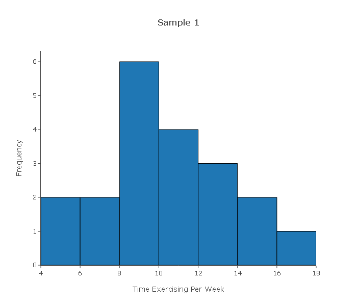
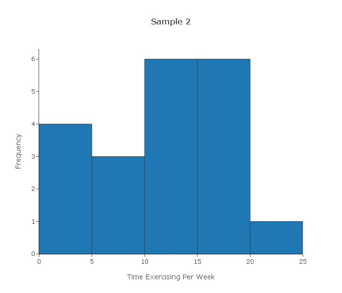
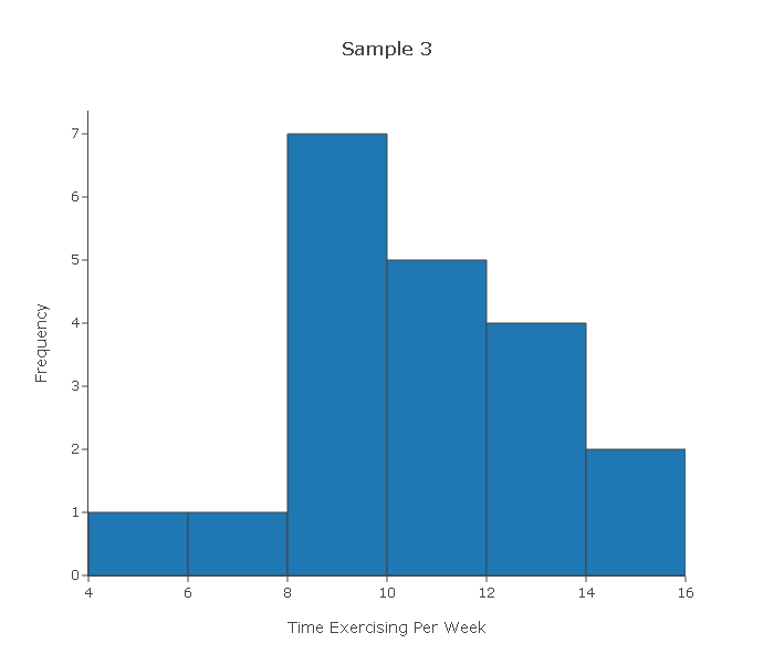
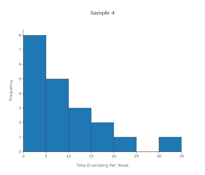
Looking at the four histograms above, comment on whether you think it would be safe to proceed with the test had those been the actual data in the problem above.

Sample 1—The histogram displays a roughly normal shape. For a sample of size 20, the shape is definitely normal enough for us to assume that the variable varies normally in the population and therefore it is safe to proceed with the test.

Sample 2—The histogram displays a distribution that is slightly skewed and does not have any outliers. The histogram, therefore, does not give us any reason to be concerned that for a sample of size 20 the Central Limit Theorem will not kick in. We can therefore proceed with the test.

Sample 3—The distribution does not have any "special" shape, and has one small outlier which is not very extreme (although it is arguable whether you would classify it as an outlier). Again, the histogram does not give us any reason to be concerned that for a sample of size 20 the Central Limit Theorem will not kick in. We can therefore proceed with the test.

Sample 4—The distribution is extremely skewed to the right, and has one pretty extreme high outlier. Based on this histogram, we should be cautious about proceeding with the test, because assuming that this histogram "paints" at least a rough picture of how the variable varies in the population, a sample of size 20 might not be large enough for the Central Limit Theorem to kick in and ensure that x-bar has a normal distribution.

Comment

It is always a good idea to look at the data and get a sense of their pattern regardless of whether you actually need to do it in order to assess whether the conditions are met.

This idea of looking at the data is not only relevant to the z-test, but to tests in general. In particular, we'll see that in the case where σ is unknown (which we'll discuss next) the conditions that allow us to safely use the test are the same as the conditions in this case, so the ideas of this activity directly apply to that case as well. Also, as you'll see, in the next section—inference for relationships—doing exploratory data analysis before inference will be an integral part of the process.

Use the following histogram to answer the question below. Hypothesis Testing for the Population Proportion p The sample size is 25. Using the histogram, should we proceed with a hypothesis test for the population mean?

Yes, although the sample size < 30, the distribution is not very far from normal in shape, with no outliers.

No, the sample size is not large enough.

Explanation :

Even though the sample size < 30, we can proceed if certain conditions are met such as the shape is nearly normal and there are no outliers.

Normal body temperature for healthy, at-rest human beings has always been said to be 98.6°F. A doctor has seen a lot of patients who had a lower or higher body temperature when they were not ill. He has read research that says it is actually lower. So, he collected 50 randomly selected temperatures that had a mean of 98.4°F. The standard deviation is known to be 0.35°F.
Ho: μ = 98.6
Ha: μ ≠ 98.6
Calculate the test statistic for this sample.

-4.04

4.04

Explanation :

The test statistic is (98.4 - 98.6) / (0.35 / sqrt(50)).

Each histogram in the questions below represents a random sample. We do not know if the variable is distributed normally in the population, but we want to be reasonably sure that the distribution of sample means will be normal so that we can use the z-test for testing claims about the population mean. For each histogram, choose the option that best describes how to proceed with a hypothesis test for a population mean. Hypothesis Testing for the Population Proportion p