Hypothesis Testing for the Population Mean: Confidence Intervals
Just as we did for proportions, we may examine a confidence interval to decide whether a proposed value of the population mean is plausible.
Suppose we want to test \( H_0: \mu = \mu_0 \) vs. \( H_a: \mu \neq \mu_0 \) using a significance level of \( \alpha = 0.05 \). An alternative way to perform this test is to find a 95% confidence interval for μ and make the following conclusions:
If \( \mu_0 \) falls outside the confidence interval, reject Ho.
If \( \mu_0 \) falls inside the confidence interval, do not reject Ho.
Example We'll use example 2, in which the alternative was two-sided.
Recall that we want to check whether a medication conforms to a target concentration of a chemical ingredient by testing
\( H_0 : \mu = 250 \)
\( H_a : \mu \neq 250 \)
We assume that \( \sigma = 12 \), and in a sample of size n = 100 we obtained a sample mean of \( \overline{x} = 247 \).
A 95% confidence interval for μ is \( \overline{x} \pm 2\frac{\sigma}{\sqrt{n}} = 247 \pm 2\frac{12}{\sqrt{100}} = 247 \pm 2.4 = (244.6, 249.6) \).
Since the interval does not contain 250, we reject Ho and conclude that the alternative is true: the population mean concentration differs from 250.

Beyond using the confidence interval as a quick way to carry out the two-sided test, the confidence interval can provide insight into the actual value of the population mean if Ho is rejected.
In the concentration level example, Ho was rejected, and all we could conclude about the mean concentration level of the entire shipment, μ, was that it was not 250.
The 95% confidence interval for μ (244.6, 249.4) gives us an idea of what plausible values for μ would be.
In particular, we can conclude that since the confidence interval lies below 250, at least a large portion of the shipment contains medication that is ineffective.
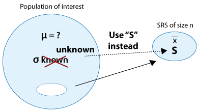
We are done with the case where the population standard deviation, σ, is known. We now move on to the more common case where σ is unknown.
- Explanation :
We are testing Ho: μ = 266 vs. Ha: μ ≠ 266. The 95% confidence interval does not cover the null value, 266, which means that at the .05 level Ho can be rejected. This is also confirmed by the p-value being 0.027, which at the 0.05 level indicates that Ho can be rejected. This is the correct answer, because this is the only output out of the three where the conclusion we make using the confidence interval and the conclusion we make using the p-value agree.
Hypothesis Testing for the Population Mean: the t Distribution
As we mentioned earlier, only in a few cases is it reasonable to assume that the population standard deviation, σ, is known. The case where σ is unknown is much more common in practice. What can we use to replace σ? If you don't know the population standard deviation, the best you can do is find the sample standard deviation, S, and use it instead of σ. (Note that this is exactly what we did when we discussed confidence intervals).
Is that it? Can we just use S instead of σ, and the rest is the same as the previous case? Unfortunately, it's not that simple, but not very complicated either.
We will first go through the four steps of the t-test for the population mean and explain in what way this test is different from the z-test in the previous case. For comparison purposes, we will then apply the t-test to a variation of the two examples we used in the previous case, and end with an activity where you'll get to carry out the t-test yourself.
Let's start by describing the four steps for the t-test:
I. Stating the hypotheses.
In this step there are no changes:
* The null hypothesis has the form: \( H_0: \mu = \mu_0 \)
(where \( \mu_0 \) is the null value).
* The alternative hypothesis takes one of the following three forms (depending on the context):
\( H_a: \mu < \mu_0 \) (one-sided)
\( H_a: \mu > \mu_0 \) (one-sided)
\( H_a: \mu \neq \mu_0 \) (two-sided)
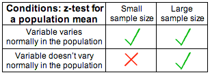
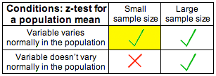
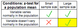
II. Checking the conditions under which the t-test can be safely used and summarizing the data.
Technically, this step only changes slightly compared to what we do in the z-test. However, as you'll see, this small change has important implications. The conditions under which the t-test can be safely carried out are exactly the same as those for the z-test:
(i) The sample is random (or at least can be considered random in context).
(ii) We are in one of the three situations marked with a green check mark in the following table (which ensure that \( \overline{X} \) is at least approximately normal):
Assuming that the conditions are met, we calculate the sample mean \( \overline{x} \) and the sample standard deviation, S (which replaces σ), and summarize the data with a test statistic. As in the z-test, our test statistic will be the standardized score of assuming that \( \mu = \mu_0 \) (Ho is true). The difference here is that we don't know σ, so we use S instead. The test statistic for the t-test for the population mean is therefore:
\( t = \frac{\overline{x} - \mu_0}{\frac{s}{\sqrt{n}}} \)
The change is in the denominator: while in the z-test we divided by the standard deviation of \( \overline{X} \), namely \( \frac{\sigma}{\sqrt{n}} \), here we divide by the standard error of \( \overline{X} \), namely \( \frac{s}{\sqrt{n}} \). Does this have an effect on the rest of the test? Yes. The t-test statistic in the test for the mean does not follow a standard normal distribution. Rather, it follows another bell-shaped distribution called the t distribution. So we first need to introduce you to this new distribution as a general object. Then, we’ll come back to our discussion of the t-test for the mean and how the t-distribution arises in that context.
The t Distribution : We have seen that variables can be visually modeled by many different sorts of shapes, and we call these shapes distributions. Several distributions arise so frequently that they have been given special names, and they have been studied mathematically. So far in the course, the only one we’ve named is the normal distribution, but there are others. One of them is called the t distribution.
The t distribution is another bell-shaped (unimodal and symmetric) distribution, like the normal distribution; and the center of the t distribution is standardized at zero, like the center of the normal distribution.
Like all distributions that are used as probability models, the normal and the t distribution are both scaled, so the total area under each of them is 1.
So how is the t distribution fundamentally different from the normal distribution?
The spread.
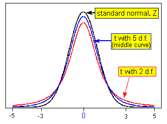
The following picture illustrates the fundamental difference between the normal distribution and the t distribution:
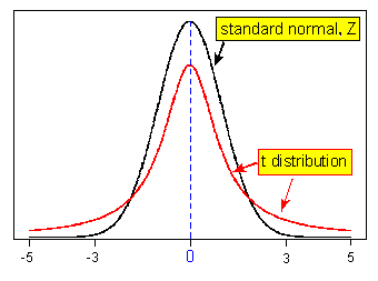
You can see in the picture that the t distribution has slightly less area near the expected central value than the normal distribution does, and you can see that the t distribution has correspondingly more area in the "tails" than the normal distribution does. (It’s often said that the t distribution has "fatter tails" or "heavier tails" than the normal distribution.)
This reflects the fact that the t distribution has a larger spread than the normal distribution. The same total area of 1 is spread out over a slightly wider range on the t distribution, making it a bit lower near the center compared to the normal distribution, and giving the t distribution slightly more probability in the ‘tails’ compared to the normal distribution.
Therefore, the t distribution ends up being the appropriate model in certain cases where there is more variability than would be predicted by the normal distribution. One of these cases is stock values, which have more variability (or "volatility," to use the economic term) than would be predicted by the normal distribution.
There’s actually an entire family of t distributions. They all have similar formulas (but the math is beyond the scope of this introductory course in statistics), and they all have slightly "fatter tails" than the normal distribution. But some are closer to normal than others. The t distributions that are closer to normal are said to have higher "degrees of freedom" (that’s a mathematical concept that we won’t use in this course, beyond merely mentioning it here). So, there’s a t distribution "with one degree of freedom," another t distribution "with 2 degrees of freedom" which is slightly closer to normal, another t distribution "with 3 degrees of freedom." which is a bit closer to normal than the previous ones, and so on.
The following picture illustrates this idea with just a couple of t distributions (note that “degrees of freedom” is abbreviated "d.f." on the picture):
- Explanation :
Indeed, the t distribution is more spread out than the Z distribution and, therefore, values that are further away from the mean (0) are more likely. In particular, under the t distribution it is more likely to get values that are above 3 than under the Z distribution. Visually, you can see that the t distribution has heavier tails and, therefore, the area under the t distribution to the right of 3 is larger than the area to the right of 3 under the Z distribution
- Explanation :
Indeed, since the t distribution has heavier tails, the area under the t distribution to the right of 1.645 would be larger than 0.05. The 95th percentile of the t distribution, therefore, must be to the right of, or larger than, 1.645.
- Explanation :
Indeed, the t distribution is more spread out than the Z distribution and, therefore, values that are further away from the mean (0) are more likely on the t distribution. In particular, getting values of less than a score of -2 is more likely with the t distribution than with the Z distribution. Visually, this is because the t distribution has "fatter tails" and, thus, there is more area to the left of -2 under the t distribution than under the Z distribution
- Explanation :
The t distribution is more spread out than the Z distribution and therefore the tail probabilities above 1 and below -1 are larger under the t distribution. As a result, the probability of getting values between -1 and 1 is smaller under the t distribution than it is under the Z distribution. Visually, the figure above shows that the area between the two blue lines is smaller under the t distribution compared to the area under the Z distribution.
Hypothesis Testing for the Population Mean: t score
Recall that we were discussing the situation of testing for a mean, in the case when σ is unknown. We’ve seen previously that when σ is known, the test statistic is \( z = \frac{\overline{x} - \mu_0}{\frac{\sigma}{\sqrt{n}}} \) (note the σ (σ) in the formula), which follows a normal distribution. But when σ is unknown, the test statistic in the test for a mean becomes \( t = \frac{\overline{x} - \mu_0}{\frac{s}{\sqrt{n}}} \) (note the use of "s" in the formula, in place of the unknown σ). Here is where the t-distribution arises in the context of a test for a mean, because \( t = \frac{\overline{x} - \mu_0}{\frac{s}{\sqrt{n}}} \) (with "s" in the formula in place of the unknown σ) follows a t distribution.
Notice the only difference between the formula for the Z statistic and the formula for the t statistic: In the formula for the Z statistic, σ (the standard deviation of the population) must be known; whereas, when σ isn’t known, then "s" (the standard deviation of the sample data) is used in place of the unknown σ. That’s the change that causes the statistic to be a t statistic.
Why would this single change (using "s" in place of "σ") result in a sampling distribution that is the t distribution instead of the standard normal (Z) distribution? Remember that the t distribution is more appropriate in cases where there is more variability. So why is there more variability when s is used in place of the unknown σ?
Well, remember that σ (σ) is a parameter (it’s the standard deviation of the population), whose value therefore never changes. Whereas, s (the standard deviation of the sample data) varies from sample to sample, and therefore it’s another source of variation. So, using s in place of σ causes the sampling distribution to be the t distribution because of that extra source of variation:
In the formula \( z = \frac{\overline{x} - \mu_0}{\frac{s}{\sqrt{n}}} \), the only source of variation is the sampling variability of the sample mean \( \overline{X} \) (none of the other terms in that formula vary randomly in a given study);
Whereas in the formula \( t = \frac{\overline{x} - \mu_0}{\frac{\sigma}{\sqrt{n}}} \), there are two sources of variation: One source is the sampling variability of the sample mean \( \overline{X} \); The other source is the sampling variability of sample standard deviation s.
So, in a test for a mean, if σ isn’t known, then s is used in place of the unknown σ and that results in the test statistic being a t score.
The t score, in the context of a test for a mean, is summarized by the following figure:
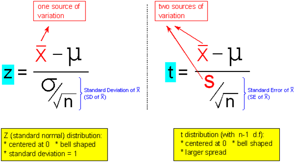
In fact, the t score that arises in the context of a test for a mean is a t score with (n – 1) degrees of freedom. Recall that each t distribution is indexed according to "degrees of freedom." Notice that, in the context of a test for a mean, the degrees of freedom depend on the sample size in the study. Remember that we said that higher degrees of freedom indicate that the t distribution is closer to normal. So in the context of a test for the mean, the larger the sample size, the higher the degrees of freedom, and the closer the t distribution is to a normal z distribution. This is summarized with the notation near the bottom on the following image:
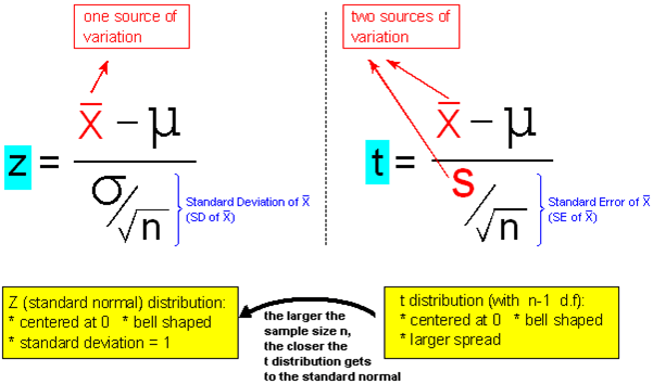
As a result, in the context of a test for a mean, the effect of the t distribution is most important for a study with a relatively small sample size.
We are now done introducing the t distribution. What are implications of all of this?
1. The null distribution of our t-test statistic: \( t = \frac{\overline{x} - \mu_0}{\frac{\sigma}{\sqrt{n}}} \) is the t distribution with (n-1) d.f. In other words, when Ho is true (i.e., when \( \mu = \mu_0 \) ), our test statistic has a t distribution with (n-1) d.f., and this is the distribution under which we find p-values.
2. For a large sample size (n), the null distribution of the test statistic is approximately Z, so whether we use t(n - 1) or Z to calculate the p-values should not make a big difference. Here is another practical way to look at this point. If we have a large n, our sample has more information about the population. Therefore, we can expect the sample standard deviation s to be close enough to the population standard deviation, σ, so that for practical purposes we can use s as the known σ, and we're back to the z-test.
Hypothesis Testing for the Population Mean: Finding the p-value for t
The p-value of the t-test is found exactly the same way as it is found for the z-test, except that the t distribution is used instead of the Z distribution, as the figures below illustrate.
Comment : Even though tables exist for the different t distributions, we will only use software to do the calculation for us.
\( H_a: \mu < \mu_0 \rightarrow p-value = P(t(n-1) \leq t) \)
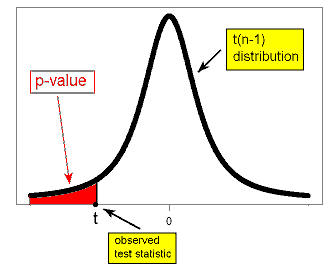
\( H_a: \mu > \mu_0 \rightarrow p-value = P(t(n-1) \geq t) \)
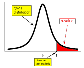
\( Ha: \mu \neq \mu_0 \rightarrow p-value = P(t(n-1) \leq -|t|) + P(t(n-1) \geq |t|) = 2P(t(n-1) \geq |t|) \)
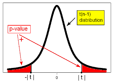
Comment : Note that due to the symmetry of the t distribution, for a given value of the test statistic t, the p-value for the two-sided test is twice as large as the p-value of either of the one-sided tests. The same thing happens when p-values are calculated under the t distribution as when they are calculated under the Z distribution.
4. Drawing Conclusions As usual, based on the p-value (and some significance level of choice) we assess the significance of results, and draw our conclusions in context.
To summarize:
The main difference between the z-test and the t-test for the population mean is that we use the sample standard deviation s instead of the unknown population standard deviation σ. As a result, the p-values are calculated under the t distribution instead of under the Z distribution. Since we are using software, this doesn't really impact us practically. However, it is important to understand what is going on behind the scenes, and not just use the software mechanically.
Hypothesis Testing for the Population Mean: Summary of t test
For comparison purposes, we use a modified version of the two problems we used in the previous case. We first introduce the modified versions and explain the changes.
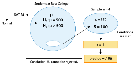
Example: 1 The SAT is constructed so that scores have a national average of 500. The distribution is close to normal. The dean of students of Ross College suspects that in recent years the college attracts students who are more quantitatively inclined. A random sample of 4 students entering Ross college had an average math SAT (SAT-M) score of 550, and a sample standard deviation of 100. Does this provide enough evidence for the dean to conclude that the mean SAT-M of all Ross College students is higher than the national mean of 500?
Here is a figure that represents this example where the changes are marked in blue:
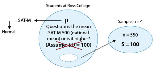
Note that the problem was changed so that the population standard deviation (which was assumed to be 100 before) is now unknown, and instead we assume that the sample of 4 students produced a sample mean of 550 (no change) and a sample standard deviation of s=100. (Sample standard deviations are never such nice rounded numbers, but for the sake of comparison we left it as 100.) Note that due to the changes, the z-test for the population mean is no longer appropriate, and we need to use the t-test.
Example: 2
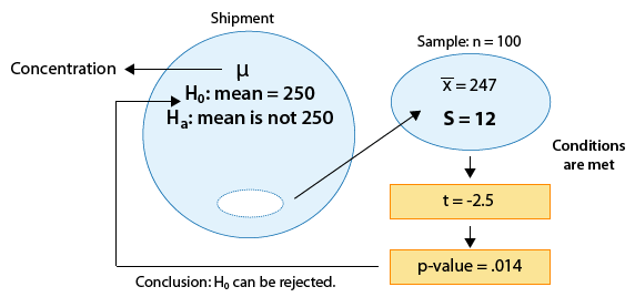
A certain prescription medicine is supposed to contain an average of 250 parts per million (ppm) of a certain chemical. If the concentration is higher than this, the drug may cause harmful side effects; if it is lower, the drug may be ineffective. The manufacturer runs a check to see if the mean concentration in a large shipment conforms to the target level of 250 ppm or not. A simple random sample of 100 portions is tested, and the sample mean concentration is found to be 247 ppm with a sample standard deviation of 12 ppm. Again, here is a figure that represents this example where the changes are marked in blue:
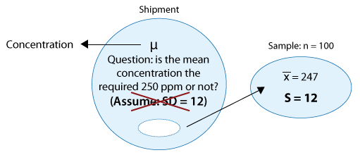
The changes are similar to example 1: we no longer assume that the population standard deviation is known, and instead use the sample standard deviation of 12. Again, the problem was thus changed from a z-test problem to a t-test problem.
However, as we mentioned earlier, due to the large sample size (n = 100) there should not be much difference whether we use the z-test or the t-test. The sample standard deviation, s, is expected to be close enough to the population standard deviation \( \sigma \) .
Example 1:
1. There are no changes in the hypotheses being tested: \( H_0: \mu = 500 \) \( H_a: \mu > 500 \)
2. The conditions that allow us to use the t-test are met since:
(i) The sample is random.
(ii) SAT-M is known to vary normally in the population (which is crucial here, since the sample size is only 4).
In other words, we are in the following situation:
The test statistic is \( t = \frac{\overline{x} - \mu_0}{\frac{s}{\sqrt{n}}} = \frac{550 - 500}{\frac{100}{\sqrt{4}}} = 1 \)
The data (represented by the sample mean) are 1 standard error above the null value.
3. Finding the p-value.
Recall that in general the p-value is calculated under the null distribution of the test statistic, which,
in the t-test case, is t(n-1). In our case, in which n = 4, the p-value is calculated under the t(3) distribution:
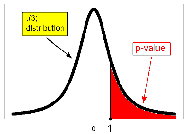
Using statistical software, we find that the p-value is 0.196. For comparison purposes, the p-value that we got when we carried out the z-test for this problem (when we assumed that 100 is the known \( \sigma \) rather the calculated sample standard deviation, s) was 0.159.
It is not surprising that the p-value of the t-test is larger, since the t distribution has fatter tails. Even though in this particular case the difference between the two values does not have practical implications (since both are large and will lead to the same conclusion), the difference is not trivial.
4. Making conclusions : The p-value (0.196) is large, indicating that the results are not significant. The data do not provide enough evidence to conclude that the mean SAT-M among Ross College students is higher than the national mean (500).
Here is a summary:
Example 2:
1. There are no changes in the hypotheses being tested:
\( H_0: \mu = 250 \) \( H_a: \mu \neq 250 \)
2. The conditions that allow us to use the t-test are met:
(i) The sample is random
(ii) The sample size is large enough for the Central Limit Theorem to apply and ensure the normality of . In other words, we are in the following situation:
The test statistic is: \( t = \frac{\overline{x} - \mu_0}{\frac{s}{\sqrt{n}}} = \frac{247 - 250}{\frac{12}{\sqrt{100}}} = -2.5 \)
The data (represented by the sample mean) are 2.5 standard errors below the null value.
3. Finding the p-value.
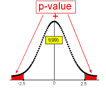
To find the p-value we use statistical software, and we calculate a p-value of 0.014 with a 95% confidence interval of (244.619, 249.381). For comparison purposes, the output we got when we carried out the z-test for the same problem was a p-value of 0.012 with a 95% confidence interval of (244.648, 249.352).
Note that here the difference between the p-values is quite negligible (0.002). This is not surprising, since the sample size is quite large (n = 100) in which case, as we mentioned, the z-test (in which we are treating s as the known \( \sigma \) ) is a very good approximation to the t-test. Note also how the two 95% confidence intervals are similar (for the same reason).
4. Conclusions:
The p-value is small (0.014) indicating that at the 5% significance level, the results are significant. The data therefore provide evidence to conclude that the mean concentration in entire shipment is not the required 250.
Here is a summary:
Comments
1. The 95% confidence interval for \( \mu \) can be used here in the same way it is used when \( \sigma \) is known: either as a way to conduct the two-sided test (checking whether the null value falls inside or outside the confidence interval) or following a t-test where Ho was rejected (in order to get insight into the value of \( \mu \) ).
2. While it is true that when \( \sigma \) is unknown and for large sample sizes the z-test is a good approximation for the t-test, since we are using software to carry out the t-test anyway, there is not much gain in using the z-test as an approximation instead. We might as well use the more exact t-test regardless of the sample size.
Let's Summarize
1. In hypothesis testing for the population mean \( \mu \), we distinguish between two cases:
I. The less common case when the population standard deviation \( \sigma \) is known.
II. The more practical case when the population standard deviation is unknown and the sample standard deviation (s) is used instead.
2. In the case when \( \sigma \) is known, the test for \( \mu \) is called the z-test, and in case when \( \sigma \) is unknown and s is used instead, the test is called the t-test.
3. In both cases, the null hypothesis is: \( H_0 : \mu = \mu_0 \) and the alternative, depending on the context, is one of the following: \( H_a : \mu < \mu_0 \), or \( H_a : \mu > \mu_0 \), or \( H_a : \mu \neq \mu_0 \)
4. Both tests can be safely used as long as the following two conditions are met:
(i) The sample is random (or can at least be considered random in context).
(ii) Either the sample size is large (n > 30) or, if not, the variable of interest can be assumed to vary normally in the population.
5. In the z-test, the test statistic is: \( z = \frac{\overline{X} - \mu_0}{\frac{\sigma}{\sqrt{n}}} \) whose null distribution is the standard normal distribution (under which the p-values are calculated).
6. In the t-test, the test statistic is: \( t = \frac{\overline{X} - \mu_0}{\frac{s}{\sqrt{n}}} \) whose null distribution is t(n - 1) (under which the p-values are calculated).
7. For large sample sizes, the z-test is a good approximation for the t-test.
8. Confidence intervals can be used to carry out the two-sided test \( H_0: \mu = \mu_0 vs. H_a : \mu \neq \mu_0 \) , and in cases where Ho is rejected, the confidence interval can give insight into the value of the population mean ().
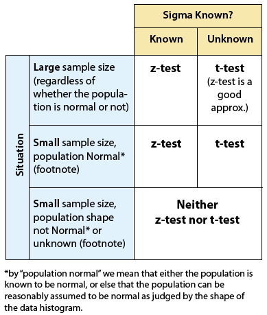
9. Here is a summary of which test to use under which conditions:
- Explanation :
Indeed, the problem description does not assume that the population standard deviation is known, and, therefore, the t-test is used.
- Explanation :
Indeed, since, based on the p-value, we cannot reject Ho at the 0.05 significance level, the 95% confidence interval must include 12.5 as a plausible value. Also the sample mean 12.008 is exactly the midpoint between 11.439 (the lower limit of the confidence interval) and 12.577, as it should be.
- Explanation :
Since the p-value of the one-sided test is 0.09 / 2 = 0.045 (half the p-value of the two-sided test), therefore, at the 0.05 significance level, Ho can be rejected and we can conclude that the mean weekly number of hours that Internet users 50-65 years of age spend less than 12.5.
- Explanation :
In this case, σ (the population standard deviation) is unknown; the only standard deviation available was the sample standard deviation (it says "computed for the sample"), so the test could not be a z-test. Then, even though the sample size is relatively small (only five boards tested), the t-test is justified, because the population is known to be normal.
- Explanation :
If the standard deviation had been for the population (so that σ had been known), then a z-test would be justified despite the small sample size.
- Explanation :
In this case, the sample size is relatively small (only 9 boards), σ is unknown, and the population cannot be reasonably assumed to vary normally (because the data distribution is noticeably skewed). So in this case, nether the z-test nor the t-test would be justified to conduct formal statistical inference. (A different sort of test called a "non-parametric" test might be justified, but that is beyond the scope of this course.)
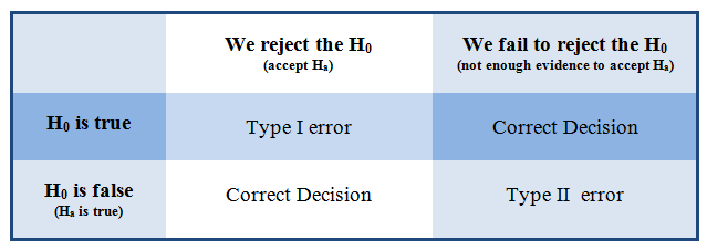
Type I and Type II Errors
Statistical investigations involve making decisions in the face of uncertainty. So there is always some chance of making a wrong decision. In hypothesis testing, the following decisions can occur:
If the null hypothesis is true and we do not reject it, it is a correct decision.
If the null hypothesis is false and we reject it, it is a correct decision.
If the null hypothesis is true, but we reject it. This is a type I error.
If the null hypothesis is false, but we fail to reject it. This is a type II error.
Type I and type II errors are not caused by mistakes. They are the result of random chance. The data provide evidence for a conclusion that is false.
Example: A Courtroom Analogy for Hypothesis Tests Defendants standing trial for a crime are considered innocent until evidence shows they are guilty. It is the job of the prosecution to present evidence that shows the defendant is guilty “beyond a reasonable doubt.” It is the job of the defense to challenge this evidence and establish a reasonable doubt. The jury weighs the evidence and makes a decision.
When a jury makes a decision, only two verdicts are possible:
Guilty: The jury concludes that there is enough evidence to convict the defendant. The evidence is so strong that there is not a reasonable doubt of the defendant’s guilt.
Not guilty: The jury concludes that there is not enough evidence to conclude beyond a reasonable doubt that the person is guilty. Notice that a verdict of “not guilty” is not a conclusion that the defendant is innocent. This verdict says only that there is not enough evidence to return a guilty verdict.
How is this like a hypothesis test?
The null hypothesis, H0, in American courtrooms is “the defendant is innocent.” The alternative hypothesis, Ha, is “the defendant is guilty.” The evidence presented in the case is the data on which the verdict is based. In a courtroom, the defendant is assumed to be innocent until proven guilty. In a hypothesis test, we assume the null hypothesis is true until the dataindicates otherwise.
The two possible verdicts are similar to the two conclusions that are possible in a hypothesis test.
Reject the null hypothesis: When we reject a null hypothesis, we accept the alternative hypothesis. This is equivalent to a guilty verdict in the courtroom. The evidence is strong enough for the jury to reject the initial assumption of innocence. In a hypothesis test, the data is strong enough for us to reject the assumption that the null hypothesis is true.
Fail to reject the null hypothesis: When we fail to reject the null hypothesis, we are delivering a “not guilty” verdict. The jury concludes that the evidence is not strong enough to reject the assumption of innocence. So the data is too weak to support a guilty verdict. We conclude the data is not strong enough to reject the null hypothesis. In other words, the data is too weak to accept the alternative hypothesis.
How does the courtroom analogy relate to Type I and Type II errors?
Type I error: The evidence leads the jury to convict an innocent person. By analogy, we reject a true null hypothesis and accept a false alternative hypothesis.
Type II error: The evidence leads the jury to declare a defendant not guilty, when he is in fact guilty. By analogy, we fail to reject a null hypothesis that is false. In other words, we do not accept an alternative hypothesis when it is really true.
It would be nice to know when each of these errors is happening when we make our decision about the null hypothesis, but statistical decisions are based on evidence gathered through sampling, and our sampling evidence will sometimes fool us. As long as we are making a decision, we will never be able to eliminate the potential for these two types of errors. Thus, we need to learn how to adjust to the consequences of making these types of errors.
- Explanation :
We fail to reject H0 when it is true.
- Explanation :
We reject H0 when it is false.
- Explanation :
A Type II error occurs when we fail to reject the H0, when it (H0) is false.
- Explanation :
With a type II error, researchers fail to reject a null hypothesis that is false. In this study, the researchers have not rejected the null hypothesis. Thus, the researchers have concluded that there is no significant difference in heart disease and breast cancer rates between the two groups. In reality, it is possible that there may have been a significant difference
- Explanation :
In a type I error, we reject a null hypothesis that is true. Here, the researchers conclude that the larger proportion of breast cancer and heart disease was statistically significant; therefore, they have rejected the null hypothesis of “no difference.
- Explanation :
We rejected the null hypothesis. With a type I error, we reject a null hypothesis that is tru
- Explanation :
It may be a type II error, because the researcher concluded based on the evidence that there is no significant difference in average salaries of men and women electricians, when in reality, there may be a significant difference between groups.
What is the probability that we will make a Type I error?
If the significance level is 5 percent (α = 0.05), then 5 percent of the time, we will reject the null hypothesis, even if it is true. Of course we will not know whether the null hypothesis is true. But if it is, the natural variability that we expect in random samples will produce “rare” results 5 percent of the time.
This makes sense, because when we create the sampling distribution, we assume the null hypothesis is true. We look at the variability in random samples selected from the population described by the null hypothesis.
Similarly, if the significance level is 1 percent, then we can expect the sample results to lead us to reject the null hypothesis 1 percent of the time. In other words, about one in 100 data sets would show “rare” results that contrast with the other 99 data sets, leading us to reject the null hypothesis. If the null hypothesis is actually true, then by chance alone, we will reject a true null hypothesis 1 percent of the time. So the probability of a type I error in this case is 1 percent.
In general, the probability of a type I error is α.
What is the probability that we will make a Type II error?
As you have just seen, the probability of a type I error is equal to the significance level, α. The probability of a type II error is much more complicated to calculate, but it is inversely related to the probability of making a type I error. Thus, reducing the chance of making a type II error causes an increase in the likelihood of a type I error.
Decreasing the Chance of Type I or Type II Error
How can we decrease the chance of a type I or type II error? Well, decreasing the chance of a type I error increases the chance of a type II error, so we must weigh the consequences of these errors before deciding how to proceed.
Recall that the probability of committing a type I error is α. Why is this? Well, when we choose a level of significance (α), we are choosing a benchmark for rejecting the null hypothesis. If the null hypothesis is true, then the probability that we will reject a true null hypothesis is α. So the smaller α is, the smaller the probability of a type I error there will be.
It is more complicated to calculate the probability of a type II error. The best way to reduce the probability of a type II error is to increase the sample size. But once the sample size is set, larger values of α will decrease the probability of a type II error while increasing the probability of a type I error.
General guidelines for choosing a level of significance:
If the consequences of a type I error are more serious, choose a small level of significance (α).
If the consequences of a type II error are more serious, choose a larger level of significance (α). But remember that the level of significance is the probability of committing a type I error.
In general, we choose the largest level of significance that we can tolerate as the chance of making a type I error.
Note: It is not always the case that one type of error is worse than the other.
- Explanation :
They could increase the sample size, as that is the best way to reduce the likelihood of a type II error.
- Explanation :
They could choose a 0.01 significance level instead of a 0.05 significance level, as this would reduce the probability of making a type I error from 5 percent to 1 percent.
- Explanation :
They could choose a 0.01 significance level instead of a 0.05 significance level, which would decrease the chance of making a type I error from 5 percent to 1 percent.
- Explanation :
Increasing the sample size is the best way to reduce the likelihood of a type II error.
- Explanation :
Increasing the sample size decreases the change of type II error but increases the chance of type I error. Choosing a smaller significance level reduces the chance of type I error but increases the chance of type II error.
Wrap-Up (Type I and Type II Errors)
It is important to remember to take into consideration the possibility of the occurrence of Type I or Type II error, when drawing conclusions from hypothesis tests. Thus:
Whenever there is a failure to reject the null hypothesis, it is possible that a Type II error has occurred.
Thus, it is concluded from the results of the study, that there are no significant differences, even though, in reality, there are significant differences.
Whenever the null hypothesis is rejected, it is possible that a Type I error has been committed.
That is, it is concluded from the results of the study, that there are significant differences, when, in reality, there are no differences.
However, it is not possible to know when either Type I or Type II error has occurred.