• In the previous Inference sections we performed inference for one variable. More specifically, we learned about inference for the population proportion p (when the variable of interest is categorical) and inference for the population mean μ (when the variable of interest is quantitative). In the previous Inference sections we were also exposed to the following three forms of inference which will continue to be central as we move forward in the course:




• Point estimation—estimating an unknown parameter with a single value that is computed from the sample.




1. Interval estimation—estimating an unknown parameter by an interval of plausible values. To each such interval we attach a level of confidence that indeed the interval captures the value of the unknown parameter and hence the name confidence intervals.




2. Hypothesis testing—a four-step process in which we are assessing evidence provided by the data in favor or against some claim about the population parameter.




• Our next (and final) goal for this course is to perform inference about relationships between two variables in a population, based on an observed relationship between variables in a sample. Here is what the process looks like:




• 




• We are interested in studying whether a relationship exists between the variables X and Y in a population of interest. We choose a random sample and collect data on both variables from the subjects. Our goal is to determine whether these data provide strong enough evidence for us to generalize the observed relationship in the sample and conclude (with some acceptable and agreed-upon level of uncertainty) that a relationship between X and Y exists in the entire population.




• The primary inference form that we will use in this module, then, is hypothesis testing. Conceptually, across all the inferential methods that we will learn, we'll test some form of:




• 




• (We will also discuss point and interval estimation, but our discussion about these forms of inference will be framed around the test.)




• Recall that in the module about examining the relationship between two variables in the Exploratory Data Analysis unit, our discussion was framed around the role-type classification table. This part of the course will be structured exactly in the same way.




• In other words, we will go through 3 sections corresponding to cases C→Q, C→C, and Q→Q in the table below.




• 




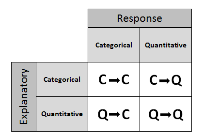
• In total, we will introduce 5 inferential methods: three in case C→Q (corresponding to a division of this case into 3 sub-cases) and one in each of the cases C→C and Q→Q.




• Unlike the previous part of the course on Inference for One Variable, where we discussed in some detail the theory behind the machinery of the test (such as the null distribution of the test statistic, under which the p-values are calculated), in the 5 inferential procedures that we will introduce in Inference for Relationships, we will discuss much less of that kind of detail. The principles are the same, but the details behind the null distribution of the test statistic (under which the p-value is calculated) become more complicated and require knowledge of theoretical results that are definitely beyond the scope of this course.




• Instead, within each of the five inferential methods we will focus on:




1. When the inferential method is appropriate for use.




2. Under what conditions the procedure can safely be used.




3. The conceptual idea behind the test (as it is usually captured by the test statistic).




4. How to use software to carry out the procedure in order to get the p-value of the test.




5. Interpreting the results in the context of the problem.




• Also, we will continue to introduce each test according to the four-step process of hypothesis testing. We are now ready to start with Case C→Q.

• Recall the role-type classification table framing our discussion on inference about the relationship between two variables.




• 




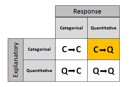
• We start with case C→Q, where the explanatory variable is categorical and the response variable is quantitative. Recall that in the Exploratory Data Analysis unit, examining the relationship between X and Y in this case amounts, in practice, to comparing the distributions of the (quantitative) response Y for each value (category) of the explanatory X. To do that, we used side-by-side boxplots (each representing the distribution of Y in one of the groups defined by X), and supplemented the display with the corresponding descriptive statistics.




• What will we do in inference? To understand the logic, we'll start with an example and then generalize.




• Example: GPA and Year in College Say that our variable of interest is the GPA of college students in the United States. From the previous module we know that since GPA is quantitative, we do inference on μ, the (population) mean GPA among all U.S. college students. Since this module is about relationships, let's assume that what we are really interested in is not simply GPA, but the relationship between:




1. X : year in college (1 = freshmen, 2 = sophomore, 3 = junior, 4 = senior) and




2. Y : GPA




• In other words, we want to explore whether GPA is related to year in college. The way to think about this is that the population of U.S. college students is now broken into 4 sub-populations: freshmen, sophomores, juniors and seniors. Within each of these four groups, we are interested in the GPA.




• The inference must therefore involve the 4 sub-population means:




1. μ1 : mean GPA among freshmen in the United States.




2. μ2 : mean GPA among sophomores in the United States




3. μ3 : mean GPA among juniors in the United States




4. μ4 : mean GPA among seniors in the United States




• It makes sense that the inference about the relationship between year and GPA has to be based on some kind of comparison of these four means. If we infer that these four means are not all equal (i.e., that there are some differences in GPA across years in college) then that's equivalent to saying GPA is related to year in college. Let's summarize this example with a figure:




• 




• In general, then, making inferences about the relationship between X and Y in Case C→Q boils down to comparing the means of Y in the sub-populations, which are created by the categories defined in X (say k categories). The following figure summarizes this:




• 




• As the introduction to this module mentioned, we will learn three inferential methods in Case C→Q, corresponding to a sub-division of this case. First we will distinguish between cases where the explanatory X has only two categories (k = 2), and cases where X has more than two categories (k > 2). In other words, we will look separately at cases where we are comparing two sub-population means:




• 




• and cases where we are comparing more than 2 sub-population means:




• 




• For example, if we are interested in whether GPA (Y) is related to gender (X), this is a case where k = 2 (since gender has only two categories: M, F), and the inference will boil down to comparing the mean GPA in the sub-population of males to that in the sub-population of females. On the other hand, in the example we looked at earlier, the relationship between GPA (Y) and year (X) is a case where k > 2 or more specifically, k = 4 (since year has four categories). In terms of inference, these two examples will be treated differently!

• Furthermore, within the sub-case of comparing two means (i.e., examining the relationship between X and Y, when X has only two categories) we will distinguish between two (sub-sub) cases.




• Here, the distinction is somewhat subtle, and has to do with how the samples from each of the two sub-populations we're comparing are chosen.




• In other words, what study design will be implemented. We have learned that many experiments, as well as observational studies, make a comparison between two groups (sub-populations) in order to see how responses differ for the two possible categorical values.




• In some cases, one group (sub-population 1) has one categorical value, and another independent group (sub-population 2) has the other value. Independent samples are then taken from each group for comparison.




• 




• In other cases, a matched pairs sample design may be used, where each observation in one sample is matched/paired/linked with an observation in the other sample. These are sometimes called "dependent samples."




• 




• Matching could be by person (if the same person is measured twice), or could actually be a pair of individuals who belong together in a relevant way (husband and wife, siblings). In this design, then, the same individual or a matched pair of individuals is used to make two measurements of the response—one for each of the two categorical values.




• Comment Note that in the first figure, where the samples are independent, the sample sizes of the two independent samples need not be the same (and thus we used n1 and n2 to indicate the two sample sizes). On the other hand, it is obvious from the design that in the matched pairs the sample sizes of the two samples must be the same (and thus we used n for both).




• Example The department of motor vehicles wants to check whether drivers are impaired after drinking two beers. Consider the following two designs:




• The reaction times (measured in seconds) in an obstacle course are measured for a group of 10 drivers who had no beer. Two beers are given to each of a different group of 9 drivers, and their reaction times on the same obstacle course are measured. (In practice, this was done by selecting a random sample of 19 drivers and randomly assigning them to one of the two groups. The random assignment guarantees, at least in theory, that the two groups are independent).




• 




• The reaction times (measured in seconds) in an obstacle course are measured for 8 randomly selected drivers before and then after the consumption of two beers.




• 




• In the first design, we have two independent samples, and the second design is a matched-pairs design, since each individual was measured twice, once before and once after. The two figures highlight the main difference between the two designs. As we'll see, when we have two independent samples, the comparison of the reaction times is a comparison between two groups. In matched pairs, the comparison between the reaction times is done for each individual.

View Answer



View Answer



View Answer

• As we mentioned in the summary of the introduction to Case C→Q, the first case that we will deal with is comparing two means when the two samples are independent:




• 




• Recall that here we are interested in the effect of a two-valued (k = 2) categorical variable (X) on a quantitative response (Y). Samples are drawn independently from the two sub-populations (defined by the two categories of X), and we need to evaluate whether or not the data provide enough evidence for us to believe that the two sub-population means are different.




• In other words, our goal is to test whether the means μ1 and μ2 (which are the means of the variable of interest in the two sub-populations) are equal or not, and in order to do that we have two samples, one from each sub-population, which were chosen independently of each other. As the title of this part suggests, the test that we will learn here is commonly known as the two-sample t-test. As the name suggests, this is a t-test, which as we know means that the p-values for this test are calculated under some t distribution. Here is how this part is organized.




• We first introduce our leading example, and then go in detail through the four steps of the two-sample t-test, illustrating each step using our example.




• NOTE... Up until now, we have been dividing our population into sub-populations, then sampling from these sub-populations.




• From now on, instead of calling them sub-populations, we will usually call the groups we wish to compare population 1, population 2, and so on. These two descriptions of the groups we are comparing can be used interchangeably.




• Example What is more important to you — personality or looks?




• This question was asked of a random sample of 239 college students, who were to answer on a scale of 1 to 25. An answer of 1 means personality has maximum importance and looks no importance at all, whereas an answer of 25 means looks have maximum importance and personality no importance at all. The purpose of this survey was to examine whether males and females differ with respect to the importance of looks vs. personality.




• The data have the following format:




• Score (Y)	Gender (X)
  15	Male
  13	Female
  10	Female
  12	Male
  14	Female
  14	Male
  6	Male
  17	Male
  etc.




• The format of the data reminds us that we are essentially examining the relationship between the two-valued categorical variable, gender, and the quantitative response, score. The two values of the categorical explanatory variable define the two populations that we are comparing — males and females. The comparison is with respect to the response variable score. Here is a figure that summarizes the example:




• 




• Comments: Note that this figure emphasizes how the fact that our explanatory is a two-valued categorical variable means that in practice we are comparing two populations (defined by these two values) with respect to our response Y.




• Note that even though the problem description just says that we had 239 students, the figure tells us that there were 85 males in the sample, and 150 females.




• Following up on comment 2, note that 85 + 150 = 235 and not 239. In these data (which are real) there are four "missing observations"—4 students for which we do not have the value of the response variable, "importance." This could be due to a number of reasons, such as recording error or nonresponse. The bottom line is that even though data were collected from 239 students, effectively we have data from only 235. (Recommended: Go through the data file and note that there are 4 cases of missing observations: students 34, 138, 179, and 183).




• We will now introduce the two-sample t-test by going through its four steps.




• Many Students Wonder ... Question: Does it matter which population we label as population 1 and which as population 2? Answer: No, it does not matter as long as you are consistent, meaning that you do not switch labels in the middle. Keeping track of how you label the populations is important in stating the hypotheses and in the interpretation of the results. In our example, it would have been fine to make population 1 be the males, and population 2 be the females. (We'll say more about this in the Learn By Doing activity)

• The Two-Sample t-Test Here again is the general situation which requires us to use the two-sample t-test:




• 




• Our goal is to compare the means μ1 and μ2 based on the two independent samples.




• Step 1: Stating the Hypotheses The hypotheses represent our goal, comparing the means: μ1 and μ2 .




• The null hypothesis has the form: \( H_0: \mu_1 - \mu_2 = 0 \) (which is the same as \( H_0 : \mu_1 = \mu_2 \) )




• The alternative hypothesis takes one of the following three forms (depending on the context): \( H_a: \mu_1 - \mu_2 < 0 \) (which is the same as \( H_a: \mu_1 < \mu_2 \) ) (one-sided)




• \( H_a: \mu_1 - \mu_2 > 0 \) (which is the same as \( H_a: \mu_1 > \mu_2 \) ) (one-sided)




• \( H_a: \mu_1 - \mu_2 \neq 0 \) (which is the same as \( H_a: \mu_1 \neq \mu_2 \) ) (two-sided)




• Note that the null hypothesis claims that there is no difference between the means, which can either represented as the difference is 0 (no difference), or as its (algebraically and conceptually) equivalent, \( \mu_1 = \mu_2 \) (the means are equal). Either way, conceptually, Ho claims that there is no relationship between the two relevant variables.




• The first way of writing the hypotheses (using a difference between the means) will be easier to use when (in the future) we look for a difference that is not 0.




• Each one of the three alternatives claims that there is a difference between the means. The two one-sided alternatives specify the nature of the difference; either negative, indicating that μ1 is smaller than μ2, or positive, indicating that μ1 is larger than μ2. The two-sided alternative, as usual, is more general and simply claims that a difference exists. As before, it should be clear from the context of the problem which of the three alternatives is appropriate.




• Comment Note that our parameter of interest in this case (the parameter about which we are making an inference) is the difference between the means \( \mu_1 - \mu_2 \) , and that the null value is 0.




• Example Recall that the purpose of this survey was to examine whether the opinions of females and males differ with respect to the importance of looks vs. personality. The hypotheses in this case are therefore:




• \( H_0: \mu_1 - \mu_2 = 0, H_a: \mu_1 - \mu_2 \neq 0 \)




• where μ1 represents the mean importance for females and μ2 represents the mean importance for males.




• It is important to understand that conceptually, the two hypotheses claim:




• Ho: Score (of looks vs. personality) is not related to gender




• Ha: Score (of looks vs. personality) is related to gender




• Scenario: Pregnancy and Smoking In order to check the claim that the pregnancy length of women who smoke during pregnancy is shorter, on average, than the pregnancy length of women who do not smoke, a random sample of 35 pregnant women who smoke and a random sample of 35 pregnant women who do not smoke were chosen and their pregnancy lengths were recorded. Here is a figure of this example:




• 

Q.

What is the null hypothesis in this case?

μ1 - μ2 = 0

μ1 - μ2 < 0

View Answer

1. Explanation :

   Indeed, in the two-sample case, the null hypothesis is always Ho: μ1 - μ2 = 0 (which can also be written as Ho: μ1 = μ2).

Q.

Which of the following statements about the null hypothesis is correct?

The null hypothesis in this case claims that pregnancy length is related to (or affected by) whether or not the woman smokes during pregnancy.

The null hypothesis in this case claims that pregnancy length is not related to (or affected by) whether or not the woman smokes during pregnancy.

View Answer

1. Explanation :

   Ho: μ1 - μ2 = 0 claims that the mean pregnancy length of women who smoke is equal to that of women who do not smoke. In other words, the null hypothesis claims that pregnancy length is not affected by whether or not the woman smokes during pregnancy.

Q.

What is the alternative hypothesis in this case?

μ1 - μ2 < 0

μ1 - μ2 > 0

View Answer

1. Explanation :

   Indeed, we want to test the claim that the mean pregnancy length of women who smoke (μ1) is smaller than the mean pregnancy length of women who do not smoke (μ2). Therefore, the alternative hypothesis in this case is Ha: μ1 < μ2 or Ha: μ1 - μ2 < 0.

Q.

Which of the following statements about the alternative hypothesis is correct?

The alternative hypothesis in this case claims that pregnancy length is related to (or affected by) whether or not the woman smokes during pregnancy.

The alternative hypothesis in this case claims that pregnancy length is not related to (or affected by) whether or not the woman smokes during pregnancy.

View Answer

1. Explanation :

   Indeed, Ha: μ1 - μ2 < 0 claims that the mean pregnancy length of women who smoke is smaller than that of women who do not smoke. This means that pregnancy length is affected by whether or not the woman smokes during pregnancy

Two Independent Samples: Conditions and Two-Sample t-test

• Step 2: Check Conditions, and Summarize the Data Using a Test Statistic The two-sample t-test can be safely used as long as the following conditions are met:




• The two samples are indeed independent.




• We are in one of the following two scenarios:




• Both populations are normal, or more specifically, the distribution of the response Y in both populations is normal, and both samples are random (or at least can be considered as such). In practice, checking normality in the populations is done by looking at each of the samples using a histogram and checking whether there are any signs that the populations are not normal. Such signs could be extreme skewness and/or extreme outliers.




• The populations are known or discovered not to be normal, but the sample size of each of the random samples is large enough (we can use the rule of thumb that > 30 is considered large enough).




• Assuming that we can safely use the two-sample t-test, we need to summarize the data, and in particular, calculate our data summary—the test statistic.




• The two-sample t-test statistic is: \( t = \frac{(\overline{y_1} - \overline{y_2}) - 0}{\sqrt{\frac{s_1^2}{n_1} + \frac{s_2^2}{n_2}}} \)




• Where:
  \( \overline{y_1}, \overline{y_2} \) are the sample means of the samples from population 1 and population 2 respectively.
  \( s_1, s_2 \) are the sample standard deviations of the samples from population 1 and population 2 respectively.
  \( n_1, n_2 \) are the sample sizes of the two samples.




• Comment Let's see why this test statistic makes sense, bearing in mind that our inference is about \( \mu_1 - \mu_2 \).




• \( \overline{y_1} \) estimates μ1 and \( \overline{y_2} \) estimates μ2, and therefore \( \overline{y_1} - \overline{y_2} \) is what the data tell me about (or, how the data estimate)




• \( \mu_1 - \mu_2 \).




• 0 is the "null value" — what the null hypothesis, Ho, claims that \( \mu_1 - \mu_2 \) is.




• The denominator \( \sqrt{\frac{s_1^2}{n_1} + \frac{s_2^2}{n_2}} \) is the standard error of \( \overline{y_1} - \overline{y_2} \). (We will not go into the details of why this is true.)




• We therefore see that our test statistic, like the previous test statistics we encountered, has the structure: \( \frac{sample estimate - null value}{standard error} \)




• and therefore, like the previous test statistics, measures (in standard errors) the difference between what the data tell us about the parameter of interest \( \mu_1 - \mu_2 \) (sample estimate) and what the null hypothesis claims the value of the parameter is (null value).




• Example Let's first check whether the conditions that allow us to safely use the two-sample t-test are met.




• Here, 239 students were chosen and were naturally divided into a sample of females and a sample of males. Since the students were chosen at random, the sample of females is independent of the sample of males.




• Here we are in the second scenario — the sample sizes (150 and 85), are definitely large enough, and so we can proceed regardless of whether the populations are normal or not.




• In order to avoid tedious calculations, we use statistics software to find the test statistic. The output (edited) is shown below:




• 




• As you can see we highlighted the “ingredients” needed to calculate the test statistic, as well as the test statistic itself. Just for this first example, let’s make sure that we understand what these ingredients are and how to use them to find the test statistic.

View Answer



View Answer



View Answer



View Answer



View Answer



View Answer

And when we put it all together we get that indeed,

• \( t = \frac{(\overline{y_1} - \overline{y_2}) - 0}{\sqrt{\frac{s_1^2}{n_1} + \frac{s_2^2}{n_2}}} \)




• t = -4.66




• The test statistic tells us what the data tell us about \( \mu_1 - \mu_2 \). In this case that difference (10.73 - 13.33) is 4.66 standard errors below what the null hypothesis claims this difference to be (0). 4.66 standard errors is quite a lot and probably indicates that the data provide evidence against Ho.

• Outputs from statistical programs vary by software programs. This information should help you to interpret the t-test results from the different programs. Please note that, while the information will vary in setup and format from program to program, the values are the same, since the same data is used for all the printouts. In addition, the format of output will be different for other tests (ex. correlation, regression, ANOVA); thus, this information pertains only to the output for t-tests.




• As reference, here is information on the problem data that was analyzed in the printouts:




• What is more important to you — personality or looks? This question was asked of a random sample of 239 college students, who were to answer on a scale of 1 to 25. An answer of 1 means personality has maximum importance and looks no importance at all, whereas an answer of 25 means looks have maximum importance and personality no importance at all. The purpose of this survey was to examine whether males and females differ with respect to the importance of looks vs. personality.




• R Output:




1. R was used to calculate the two independent samples t-test result, using gender (Gender) as the categorical explanatory/independent variable and the importance of personality (looks) as the quantitative response/dependent variable. The data command used to produce this output is as follows:




2. 




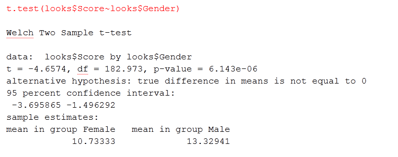
3. The top line tells us that a two sample t-test was calculated.




4. The second line tell us specifically what was analyzed (ex. data:)




5. The third line has three values:




6. t = -4.6574, which is the value of the t-statistic




7. df = 182.973, which is the degrees of freedom. It is used when determining critical value.




8. p-value = 6.143e-06, which is the exact probability of getting this value for the t-statistic. The value is written in scientific notation, which needs to be converted to get the exact probability level. Since this value ends in e-06, the decimal point needs to be moved 6 places to the left. Thus, 6.143e-06 equals 0.000006143, which is very, very small. When rounded to four decimal points, the P-value is 0.0001; thus, we can reject the null hypothesis that there is no difference between the mean score of Females and the mean score of Males on the importance of looks. The fourth line describes the alternative hypothesis. In this case, since the “true difference in means is not equal to 0;” thus, it assessing that the claim that there is a difference, but not that one group is higher or lower than the other group, which is a two-sided, two independent samples t-test.




9. The fifth line tells us that the sixth line contains the 95% confidence interval that can be used to assess the null hypothesis (H0 : μ1 - μ2 = 0). Thus, the 95% confidence interval is: (-3.695865, -1.496292). Since 0 does not fall within the 95% confidence interval, we can reject the null hypothesis that there is no difference between the mean score of Females and the mean score of Males on the importance of looks. As it should be, these results are consistent with the above results, where the P-value was used.




10. The last three lines give us information on the samples; in this case, group means.




11. mean personality score for females: 10.73333




12. mean personality score for males: 13.32941




• StatCrunch (edited) Output:




1. StatCrunch was used to produce the following three charts, with gender (Gender) as the categorical explanatory/independent variable and the importance of personality (looks) as the quantitative response/dependent variable.




2. The first chart contains summary statistics for the two samples (Females and Males) on the quantitative response/dependent variable (looks). The second chart contains the (two-sided) two independent samples t-test result, using gender (Gender) as the categorical explanatory/independent variable and the importance of personality (looks) as the quantitative response/dependent variable with the P-value method for assessing the null hypothesis.




3. The third chart contains the (two-sided) two independent samples t-test result, using gender (Gender) as the categorical explanatory/independent variable and the importance of personality (looks) as the quantitative response/dependent variable with the 95% confidence interval method for assessing the null hypothesis.




4. 




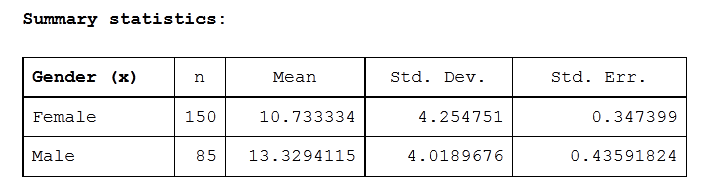
5. The above chart displays information on the characteristics of the samples.




6. The first line gives a description of the information contained in each column, while the first column tells us what information is contained in each of the rows:




1. Column 1 contains information on the x (explanatory/independent) categorical variable. In this case, there are two levels of the x variable, Gender: males and females. Thus, row 2 refers only to information on the sample of Females, while row 3 refers only to information on the sample of Males.




2. Column 2 contains information on the number of observations in each sample: 150 Females and 85 Males.




3. Column 3 contains the means for each of the samples: 10.733334 for Females and 13.3294115 for Males.




4. Column 4 contains the standard deviation for each of the samples: 4.254751 for Females and 4.0189676 for Males.




5. Column 5 contains the standard deviation of the sampling distribution (which is also known as the standard error): 0.347399 for Females and 0.43591824 for Males.




6. 




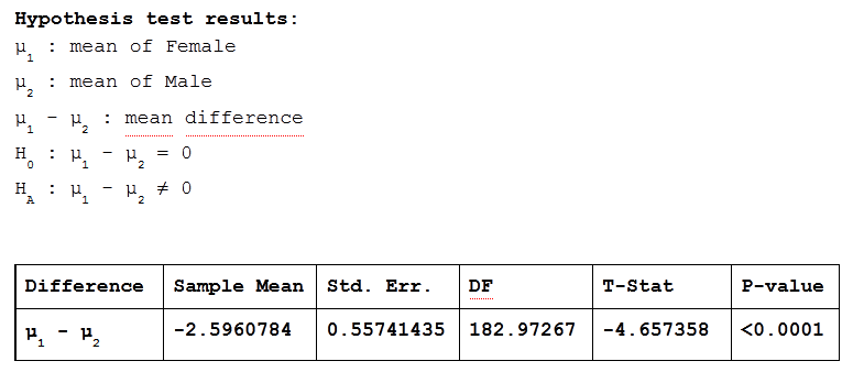
7. The above chart shows the results of the two-sided (since the alternative hypothesis is: Ha : μ1 - μ2 ≠ 0), two independent samples t-test, using the P-value method.




7. The first line gives a description of the information contained in each column:




1. Column 1 contains information on the difference that is being assessed: μ1 - μ2, where μ1 is the population mean for Females and μ2 is the population mean for Males.




2. Column 2 contains the difference between the sample means that is being assessed in the t-test. Thus, the mean from the sample of Females (10.733334) minus the mean from the sample of Males (13.3294115) or 10.7333334 - 13.3294115 = -2.5960784.




3. Column 3 contains the standard error.




4. Column 4 contains the degrees of freedom, which is based on the sample sizes and is used to determine the critical value for cutoff scores.




5. Column 5 contains the t-statistic, which is -4.657358.




6. Column 6 contains the P-value, which is < 0.0001. Thus, we can reject the null hypothesis that there is no difference between the mean score of Females and the mean score of Males on the importance of looks.




7. 




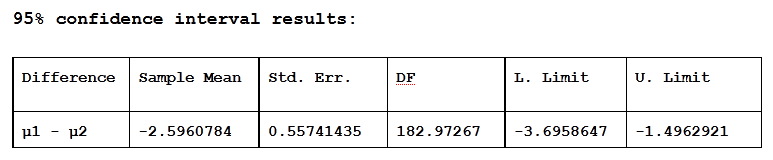
8. The above chart shows the results of the two-sided (since the alternative hypothesis is: Ha : μ1 - μ2 ≠ 0), two independent samples t-test, using 95% confidence intervals.




8. The first line gives a description of the information contained in each column:




1. Column 1 contains information on the difference that is being assessed: μ1 - μ2, where μ1 is the population mean for Females and μ2 is the population mean for Males.




2. Column 2 contains the difference between the sample means that is being assessed in the t-test. Thus, the mean from the sample of Females (10.733334) minus the mean from the sample of Males (13.3294115) or 10.7333334 - 13.3294115 = -2.5960784.




3. Column 3 contains the standard error.




4. Column 4 contains the degrees of freedom, which is based on the sample sizes and is used to determine the critical value for cutoff scores.




5. Column 5 contains the lower limit and Column 6 contains the upper limit of the 95% confidence interval that can be used to assess the null hypothesis (H0 : μ1 - μ2 = 0). Thus, the 95% confidence interval is: (-3.6958647, -1.4962921). Since 0 does not fall within the 95% confidence interval, we can reject the null hypothesis that there is no difference between the mean score of Females and the mean score of Males on the importance of looks. As it should be, these results are consistent with the results from the previous table, where the P-value was used.




• Minitab Output:




• Minitab was used to calculate the two independent samples t-test result, using gender (Gender) as the categorical explanatory/independent variable and the importance of personality (looks) as the quantitative response/dependent variable. The below chart shows the results of the two-sided (since the alternative hypothesis is: HA : μ1 - μ2 ≠ 0), two independent sample t-test, using both the P-value and 95% confidence interval to assess the null hypothesis.




• 




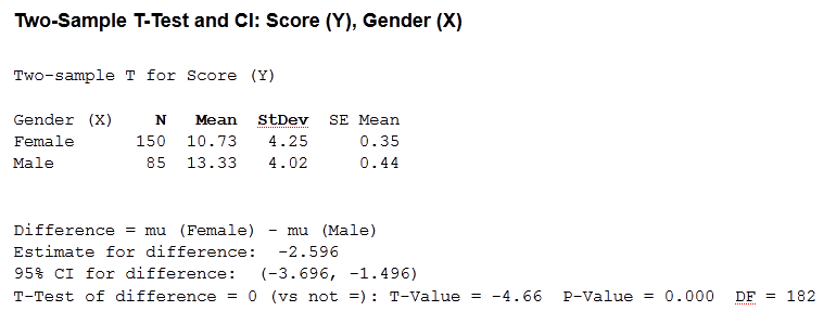
• The top line tells us that a two sample t-test was calculated, using score as the response/dependent variable and gender as the explanatory/independent variable.




• The second line tell us that the two sample t-test was calculated with score as the response/dependent variable.




• The third, fourth, and fifth lines, comprise a table of summary statistics for the response/dependent variable. The third line gives a description of the information contained in each column, while the first column tells us what information is contained in each of the rows:




1. Column 1 contains information on the x (explanatory/independent) categorical variable. In this case, there are two levels of the x variable, Gender: males and females. Thus, row 2 refers only to information on the sample of Females, while row 3 refers only to information on the sample of Males.




2. Column 2 contains information on the number of observations in each sample: 150 Females and 85 Males.




3. Column 3 contains the means for each of the samples: 10.73 for Females and 13.33 for Males.




4. Column 4 contains the standard deviation for each of the samples: 4.25 for Females and 4.02 for Males.




5. Column 5 contains the standard deviation of the sampling distribution (which is also known as the standard error): 0.35 for Females and 0.44 for Males.




• The sixth line contains information on the difference that is being assessed: μu - μu; in this case, the population mean of males is subtracted from the population mean of females.




• The seventh line the difference between the sample means that is being assessed in the t-test. Thus, the mean from the sample of Females (10.73) minus the mean from the sample of Males (13.33) or 10.73 - 13.33 = -2.596.




• The eighth line contains the 95% confidence interval that can be used to assess the null hypothesis (H0 : μ1 - μ2 = 0). Thus, the 95% confidence interval is: (-3.696, -1.496). Since 0 does not fall within the 95% confidence interval, we can reject the null hypothesis that there is no difference between the mean score of Females and the mean score of Males on the importance of looks.




• The ninth line has three values:




• T-Test of difference = 0 (vs not =): T-Value = -4.66, which tells us that this is a two-sided two sample t-test, with a t-statistic value of -4.66. P-value = 0.000, which is the exact probability of getting this value for the t-statistic. Since it is not possible to have 0 probability, the last value is changed to a 1, when reporting, and it shows that, with a P-value of 0.001, we can reject the null hypothesis that there is no difference between the mean score of Females and the mean score of Males on the importance of looks. As it should be, these results are consistent with the results from the previous line (line 8), where the 95% confidence interval was used. DF = 182, which is the degrees of freedom. It is used when determining the critical value.




• TI Calculator Output:




1. The TI calculator was used to calculate the two independent samples t-test result, using gender (Gender) as the categorical explanatory/independent variable and the importance of personality (looks) as the quantitative response/dependent variable. The below chart shows the results of the two-sided (since the alternative hypothesis is: HA : μ1≠ μ2 ), two independent sample t-test, using the P-value to assess the null hypothesis.




2. 




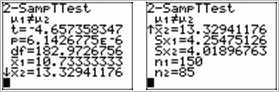
3. The top lines of both the left and right images tell us that a two sample t-test was calculated, while the second lines tell us that the alternative hypothesis is HA : μ1≠ μ2. Thus, these are the results for a two-sided two sample t-test.




4. Left Chart:




1. The third line shows the t-statistic, which is -4.657358347.




2. The fourth line shows the p-value = 6.1426775e-06, which is the exact probability of getting this value for the t-statistic. The value is written in scientific notation, which needs to be converted to get the exact probability level. Since this value ends in e-06, the decimal point needs to be moved 6 places to the left. Thus, 6.143e-06 equals 0.000006143, which is very, very small. When rounded to four decimal points, the P-value is 0.0001; thus, we can reject the null hypothesis that there is no difference between the mean score of Females and the mean score of Males on the importance of looks.




3. The fifth line contains the degrees of freedom, which is df = 182.9726756. It is used when determining critical value.




4. The sixth line contains the mean for the first sample, which is Females: 10.73333333.




5. The seventh line contains the mean for the second sample, which is Males: 13.32941176




5. Right Chart (which is a continuation of the left chart, when viewed on the calculator screen):




1. The third line contains the mean for the second sample, which is Males: 13.32941176.




2. The fourth line contains the standard deviation for the first sample, which is Females: 4.25475126.




3. The fifth line contains the standard deviation for the second sample, which is Males: 4.01896763.




4. The sixth line contains the sample size for the first sample, which is 150 Females.




5. The seventh line contains the sample size for the second sample, which is 85 Males.

• Scenario: TV Watching and Gender The purpose of this activity is to give you guided practice in checking whether the conditions that allow us to use the two-sample t-test are met.




• Background A researcher wanted to study whether or not men and women differ in the amount of time they watch TV during a week. In each of the following cases, you'll have to decide whether we can use the two-sample t-test to test this claim or not.




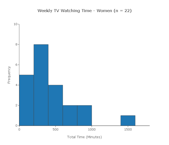
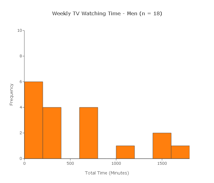
• 1. A random sample of 40 adults was chosen (22 of whom were women and 18 of whom were men). At the end of the week, each of the 40 subjects reported the total amount of time (in minutes) that he/she watched TV during that week.




• Below are two histograms to view the data for men's and women's weekly TV watching time




• 




• Can we use the two-sample t-test to test this claim?




1. Let's check the two conditions:




2. (i) Since the 40 subjects were chosen at random, we can assume that the two samples are independent.




3. (ii) Since the sample sizes (22 and 18) are not large, for the two-sample t-test to be reliably used the two populations need to be (at least close) to normal.




4. In practice, we check by looking at our two samples using histograms and making sure that we don't see any gross violation of the normality assumption. However, both histograms display clear violations of the normality assumption in the form of extreme skewness and outliers. In conclusion, the two-sample t-test cannot be reliably used.

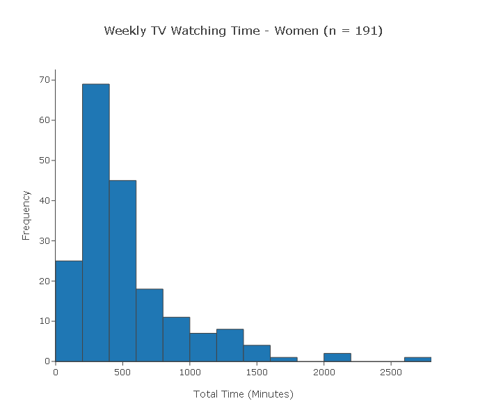
• A random sample of 400 adults was chosen (191 women and 209 men). At the end of the week, each of the 400 subjects reported the total amount of time (in minutes) that he or she watched TV during that week.




• Below are the two histograms men's and women's weekly TV watching time for this sample.




• 




• 




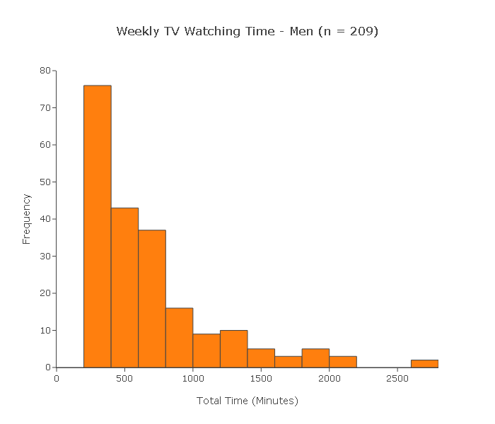
• Can we use the two-sample t-test to test this claim?




1. (i) Since the 400 subjects were chosen at random, we can assume that the two samples are independent.




2. (ii) Since the sample sizes (191 and 209) are large, we can proceed with the two-sample t-test regardless of whether the populations are normal or not. In conclusion, we can reliably use the two-sample t-test in this case.

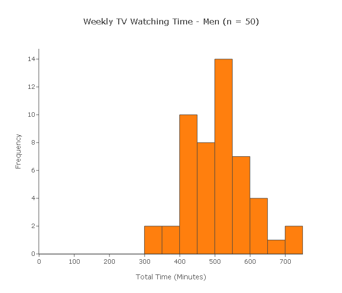
• A random sample of 25 women and another random sample of 25 men was chosen. At the end of the week, each of the 50 subjects reported the total amount of time (in minutes) that he or she watched TV during that week.




• 




• 




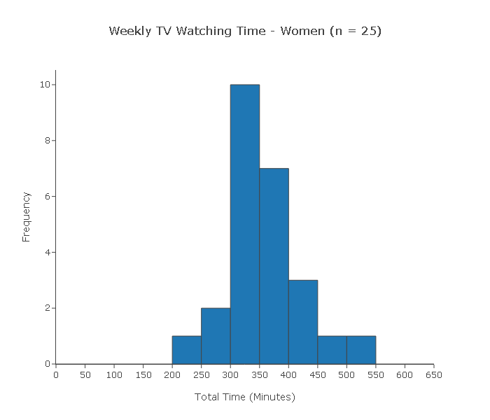
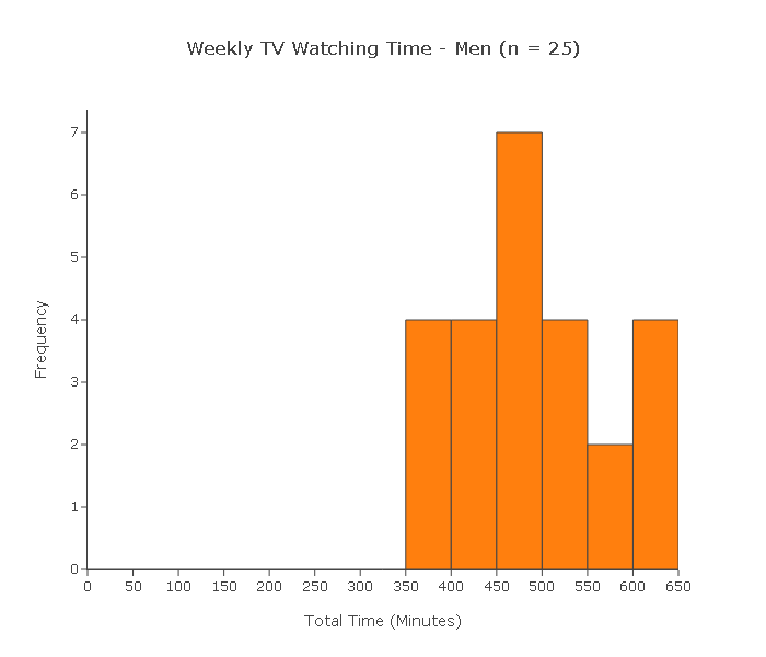
• Can we use the two-sample t-test to test this claim?




1. (i) Since each of the samples is random, we can assume that the samples are independent.




2. (ii) Since the sample sizes (both 25) are not large, for the two-sample t-test to be reliably used the two populations need to be (at least close) to normal.




3. Indeed, when we look at the histograms of the samples, we see no violations of the normality assumption. On the contrary, both histograms have a shape which is close to normal. In conclusion, we can reliably use the two-sample t-test in this case

• A random sample of 50 married couples was chosen, which was split into a sample of 50 men and a sample of 50 women. At the end of the week, each of the 100 subjects reported the total amount of time (in minutes) that he or she watched TV during that week.




• 




• 




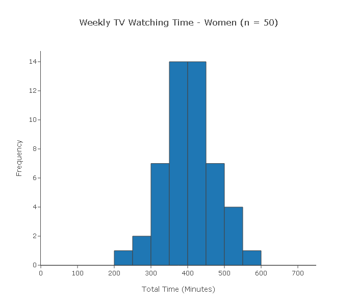
• Can we use the two-sample t-test to test this claim?




1. (i) This is a case where the two samples are not independent. Since each subject in one sample is linked (by marriage) to a subject in the other sample, these samples are dependent. The two-sample t-test is therefore not appropriate in this case.

• Step 3: Finding the p-value of the test Since our test is called the two-sample t test ,we know that the p-values are calculated under a t distribution. Indeed, it turns out that the null distribution of our test statistic is approximately t. Figuring out which one of the t distributions (in other words, how many degrees of freedom this t distribution has) is quite involved and will not be discussed here. Instead, we use a statistics package to find that the p-value in this case is 0.




• Example Here, again is the relevant output for our example:




• 




• According to the output the p-value of this test is less than 0.0001. How do we interpret this?




1. A p-value which is practically 0 means that it would be almost impossible to get data like that observed (or even more extreme) had the null hypothesis been true.




2. More specifically to our example, if there were no differences between females and males with respect to whether they value looks vs. personality, it would be almost impossible (probability approximately 0) to get data where the difference between the sample means of females and males is -2.596 (that difference is 10.733 - 13.329 = -2.596) or higher.




• Comment: Note that the output tells us that \( \overline{y_1} - \overline{y_2} \) is approximately -2.6. But more importantly, we want to know if this difference is significant. To answer this, we use the fact that this difference is 4.66 standard errors below the null value.




• Step 4: Conclusion in context As usual a small p-value provides evidence against Ho. In our case our p-value is practically 0 (which smaller than any level of significance that we will choose). The data therefore provide very strong evidence against Ho so we reject it and conclude that the mean Importance score (of looks vs personality) of males differs from that of females. In other words, males and females differ with respect to how they value looks vs. personality.




• Comments :




1. It is true that for all practical purposes all we have to do is check that the conditions which allow us to use the two-sample t-test are met, lift the p-value from the output, and draw our conclusions accordingly.




2. However, we feel that it is important to mention the test statistic for two reasons:




3. The test statistic is what's behind the scenes; based on its null distribution and its value, the p-value is calculated.




4. Apart from being the key for calculating the p-value, the test statistic is also itself a measure of the evidence stored in the data against Ho. As we mentioned, it measures (in standard errors) how different our data is from what is claimed in the null hypothesis.

• Example According to the National Health And Nutrition Examination Survey (NHANES) sponsored by the U.S. government, a random sample of 712 males between 20 and 29 years of age and a random sample of 1,001 males over the age of 75 were chosen, and the weight of each of the males was recorded (in kg). Here is a summary of the results




• 




• Do the data provide evidence that the younger male population weighs more (on average) than the older male population? (Note that here the data are given in a summarized form, unlike the previous problem, where the raw data were given.)




• Here is a figure that summarizes this example:




• 




• Note that we defined the younger age group and the older age group as population 1 and population 2, respectively, and μ1 and μ2 as the mean weight of population 1 and population 2, respectively.




• Step 1: Since we want to test whether the older age group (population 2) weighs less on average than the younger age group (population 1), we are testing: \( H_0: \mu_1 - \mu_2 = 0, H_a: \mu_1 - \mu_2 > 0 \) or equivalently, \( H_0: \mu_1 = \mu_2, H_a: \mu_1 > \mu_2 \)




• Step 2: We can safely use the two-sample t-test in this case since: The samples are independent, since each of the samples was chosen at random. Both sample sizes are very large (712 and 1,001), and therefore we can proceed regardless of whether the populations are normal or not. It is possible from these data to calculate the t-statistic of 5.31 and the p-value of 0.000. The t-value is quite large, and the p-value correspondingly small, indicating that our data are very different from what is claimed in the null hypothesis.




• Step 3: The p-value is essentially 0, indicating that it would be nearly impossible to observe a difference between the sample mean weights of 4.9 (or more) if the mean weights in the age group populations were the same (i.e., if Ho were true).




• Step 4: A p-value of 0 (or very close to it) indicates that the data provide strong evidence against Ho, so we reject it and conclude that the mean weight of males 20-29 years old is higher than the mean weight of males 75 years old and older. In other words, males in the younger age group weigh more, on average, than males in the older age group.

• Background : A study was conducted at a large state university in order to compare the sleeping habits of undergraduate students to those of graduate students. Random samples of 75 undergraduate students and 50 graduate students were chosen and each of the subjects was asked to report the number of hours he or she sleeps in a typical day. The thought was that since undergraduate students are generally younger and party more during their years in school, they sleep less, on average, than graduate students. Do the data support this hypothesis? The following figure summarizes the problem:




• 




• Note that we defined:




• μ1—the mean number of hours undergraduate students sleep in a typical day
  μ2—the mean number of hours graduate students sleep in a typical day




• State the null and alternative hypotheses that are being tested here.




• Since we want to check whether the data supports the claim that undergraduate students sleep less, on average, than graduate students, we are testing:




• H0: μ1 − μ2 = 0
  Ha: μ1 − μ2 < 0




• Explain why we can safely use the two-sample t-test in this case




1. We can safely use the two-sample t-test in this case since:




2. • Both samples are random, and therefore independent.




3. • The sample sizes (75 and 50) are quite large, and therefore we can proceed regardless of whether the populations are normal or not.




4. Comment: Before we move on to carry out the test, it is important to realize that in the two-sample problem, the data can be provided in three possible ways:




5. (i) Sample data in one column, and another column that indicates which sample the observation belongs to. Recall that this is the way the data were given in our leading example (looks vs. personality score and gender):




6. Score (Y)	Gender (X)
   15	Male
   13	Female
   10	Female
   12	Male
   14	Female
   14	Male
   6	Male
   17	Male
   ...	...




7. Note that essentially , one column contains the explanatory variable, and one contains the response. (ii) Sample data in different columns—data from each of the two samples appear in a column dedicated to that category. As you'll see, this is the way the data are provided in this example:




8. Undergraduate	Graduate
   6	8
   5	5
   3	6
   612	6
   ...	...




9. (iii) Summarized data—we are not given the actual data, but just the data summaries: sample sizes, sample means and sample standard deviations of both samples. Recall that in our second example, the data were given in this format.




10. 




11. We carry out the two-sample t-test and get the following results:




12. 




13. Based on the output, what conclusions would you draw?




1. The p-value is not small (in particular, it is larger than 0.05), indicating that it is still reasonably likely (probability 0.111) to get data like those observed, or even more extreme data, under the null hypothesis (i.e., assuming that undergraduate and graduate students have the same mean sleeping hours). Therefore, the data do not provide evidence to reject Ho, and we cannot conclude that undergraduate students sleep less, on average, than graduate students.

Previous

Next