Two Independent Samples: Confidence Interval
Confidence Interval for \( \mu_1 - \mu_2 \) (Two-Sample t Confidence Interval) So far we've discussed the two-sample t-test, which checks whether there is enough evidence stored in the data to reject the claim that \( \mu_1 - \mu_2 = 0 \) (or equivalently, that \( \mu_1 = \mu_2 \) ) in favor of one of the three possible alternatives.
If we would like to estimate \( \mu_1 - \mu_2 \) we can use the natural point estimate, \( \overline{y_1} - \overline{y_2} \) , or preferably, a 95% confidence interval which will provide us with a set of plausible values for the difference between the population means \( \mu_1 - \mu_2 \) .
In particular, if the test has rejected \( H_) : \mu_1 - \mu_2 = 0 \) , a confidence interval for \( \mu_1 - \mu_2 \) can be insightful since it quantifies the effect that the categorical explanatory variable has on the response.
Comment We will not go into the formula and calculation of the confidence interval, but rather ask our software to do it for us, and focus on interpretation.
Example Recall our leading example about the looks vs. personality score of females and males:
Here again is the output:
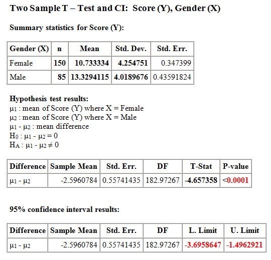
Recall that we rejected the null hypothesis in favor of the two-sided alternative and concluded that the mean score of females is different from the mean score of males. It would be interesting to supplement this conclusion with more details about this difference between the means, and the 95% confidence interval for \( \mu_1 - \mu_2 \) does exactly that.
According to the output the 95% confidence interval for \( \mu_1 - \mu_2 \) is roughly (-3.7, -1.5). First, note that the confidence interval is strictly negative suggesting that μ1 is lower than μ2 . Furthermore, the confidence interval tells me that we are 95% confident that the mean "looks vs. personality score" of females ( μ1 ) is between 1.5 and 3.7 points lower than the mean looks vs. personality score of males ( μ2 ). The confidence interval therefore quantifies the effect that the explanatory variable (gender) has on the response (looks vs personality score).
Scenario: Weight by Mens Age
The purpose of this activity is to give you guided practice in interpreting a 95% confidence interval for μ1 - μ2 following a two-sample t-test that rejected Ho. Recall our second example:
Recall that we were testing
\( H_0: \mu_1 - \mu_2 = 0, H_a: \mu_1 - \mu_2 > 0 \)
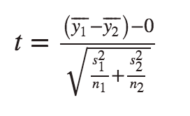
and we found using statistical software that the test statistic was 5.31 with a p-value of 0.000. Based on the small p-value, we rejected Ho and concluded that males 20-29 years old weigh more, on average, than males 75+ years old. It would be interesting to follow up this conclusion and estimate how much more males 20-29 years old weigh, on average. The 95% confidence interval for μ1 - μ2 does exactly that, and is given by the formula
\( (\overline{Y_1} - \overline{Y_2}) \pm t* \sqrt{\frac{s_1^2}{n_1} + \frac{s_2^2}{n_2}} \)
As a reminder, here again is the summary of the study results:
- Explanation :
This means that with 95% confidence, we can say that males who are 20-29 years old weigh, on average, 3.1 to 6.7 kilograms *more* than males who are 75 and older.
Two Independent Samples: Summary
Comment : As we saw in previous tests, as well as in the two-samples case, the 95% confidence interval for \( \mu_1 - \mu_2 \) can be used for testing in the two-sided case ( \( H_0 : \mu_1 - \mu_2 = 0 \) vs. \( H_a : \mu_1 - \mu_2 \neq 0 \) ):
If the null value, 0, falls outside the confidence interval, Ho is rejected
If the null value, 0, falls inside the confidence interval, Ho is not rejected
Example Let's go back to our leading example of the looks vs. personality score where we had a two-sided test.
We used the fact that the p-value is so small to conclude that Ho can be rejected. We can also use the confidence interval to reach the same conclusion since 0 falls outside the confidence interval. In other words, since 0 is not a plausible value for \( \mu_1 = \mu_2 \) we can reject Ho, which claims that \( \mu_1 - \mu_2 = 0 \) .
Scenario: Sugar Content in Fruit Juice and Soda The purpose of this activity is to help you practice the connection between the two branches of formal inference (significance testing and confidence intervals) in the context of two independent samples.
Background:
Fruit juice is often marketed as being a healthier alternative to soda. And although juice does contain vitamins, juice can also be surprisingly high in sugar. Since excess sugar from any source can play a role in diseases like obesity and diabetes, it is important to be quantitatively informed about the beverages we consume.
To compare the sugar content (in grams) between soda and 100% fruit juice, an investigation was made of 34 representative popular U.S. brands of 100% bottled juice (such as Dole, Minute Maid, Motts, Juicy Juice, Ocean Spray, Tree Top Apple, V8 Fusion, and Welch’s Grape), and 45 representative popular U.S. brands of soda pop (such as 7-Up, A&W Root Beer, Coca-Cola, Crush, Dr. Pepper, Fanta, Hawaiian Punch, Pepsi Cola, RC Cola, Sierra Mist, Schweppes Ginger Ale, and Sprite).
(Note, these are real data.)
Hypotheses: - If we let μ1 represent the mean sugar content of the population of all bottled 100% fruit juices on the market, and if we let μ2 represent the mean sugar content of the population all sodas on the market, then the significance test of interest are the hypotheses:
Null hypothesis: μ1 - μ2 = 0 ; (in other words, that there is no difference between the overall mean sugar content of on-the-market juices and on-the-market sodas, i.e., that the two beverage categories have the same overall mean sugar content).
Alternative hypothesis: μ1 - μ2 ≠ 0 ; (in other words, that there is a difference between the overall mean sugar content of on-the-market juices and on-the-market sodas, i.e., that the two beverage categories don’t have the same overall mean sugar content).
Summary statistics:
The summary of sugar content (in grams) for the two samples is as follows (remember, these are real data):
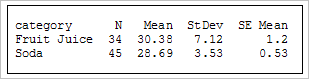
We see that the sample mean sugar content of the 34 juices was actually higher, at 30.38 grams, while the sample mean sugar content of the 45 sodas was only 28.69 grams.
The inferential question of interest is whether the slight difference is statistically significant.
Checking conditions for inference:
For the purpose of statistical inference, we will consider the drinks in the study to be random samples of all such drinks on the market.
There are two independent groups (fruit juice versus soda); and since the σs (the standard deviations of the populations) are unknown to us, our required test will be a t-test for two independent means.
To check that a t-test for two independent means is reasonably justified, we should consider the shape of the histograms as well as the sample sizes in the study.
The histograms of sugar content for the two groups are as follows:
The histogram of sugar content for the soda sample (the graph on the right) is clearly unimodal and symmetric without any outliers; that shape helps to justify the desired inference procedure. The histogram of sugar content for the juice sample (the graph on the left) isn’t quite as nice from the standpoint of justifying inference, since it’s less clearly unimodal (although still clearly symmetric) and it has one possible outlier on its left side (although not too severe an outlier); but since the sample sizes in the study were each relatively large (n1 = 34 brands of juice and n2 = 44 brands of soda) the t-test is still justified, despite the possible bimodality and possible (and not-too-severe) outlier of the juice sample.
Result of Inference:
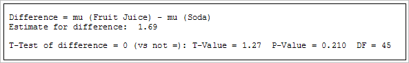
Here is the output from the formal t-test for two independent means:
Based on the output, state the appropriate formal conclusion of the test of the hypotheses
Ho: μ1 - μ2 = 0
Ha: μ1 - μ2 ≠ 0
and then briefly state the meaning of the conclusion in the context of the question regarding whether there is reason to believe that the average sugar content of all 100% fruit juices sold is any different than the average sugar content of all sodas sold.Based on the magnitude of the p-value shown in the output (p-value = 0.210), we do not reject the null hypothesis (since the p-value is relatively large).
This means that the study does not provide sufficient evidence that the average sugar content of all fruit juices sold is any different than the average sugar content of all sodas.
Follow up remarks: The conclusion is interesting for two reasons. First, we might have initially suspected (prior to the study) that sodas would have a higher average sugar content than juices; but the formal inference shows that this supposition is not supported. Second, after seeing the summary statistics (but not the inference), we saw that the sample of juices actually had slightly higher average sugar content than the sodas, so we might have then wondered if juices overall actually have a higher average sugar content than sodas; but the inferential conclusion shows that this is not supported either.
- Explanation :
The confidence interval most likely contains the true value of the difference being hypothesized about, i.e., the confidence interval should contain the value of μ1 - μ2. So, since we didn’t reject the null hypothesis, the interval in this case should contain zero, because we believe the null hypothesis (i.e., we believe that μ1 - μ2 = 0). The interval here is the only interval that contains zero, since the left-hand endpoint of the interval is negative while the right-hand endpoint of the interval is positive.
- Explanation :
Below you'll find three sample outputs of the two-sided two-sample t-test:
\( H_0: \mu_1 - \mu_2 = 0 vs. H_a: \mu_1 - \mu_2 \neq 0 \)
However, only one of the outputs could be correct (the other two contain an inconsistency). Your task is to decide which of the following outputs is the correct one.Output A:
p-value: 0.289
95% Confidence Interval: (-5.93090, -1.78572)
Output B:
p-value: 0.003
95% Confidence Interval: (-13.97384, 2.89733)
Output C:
p-value: 0.223
95% Confidence Interval: (-9.31432, 2.20505)
- Explanation :
Indeed, this is the correct output, since it is the only one out of the three in which both the confidence interval and p-value lead us to the same conclusion (as it should be). Note that 0 falls inside the 95% confidence interval for μ1 - μ2, which means that Ho cannot be rejected. Also, the p-value is large (0.223) indicating that Ho cannot be rejected.
- Explanation :
Summarize
The two sample t-test is used for comparing the means of a quantitative variable (Y) in two populations (which we initially called sub-populations).
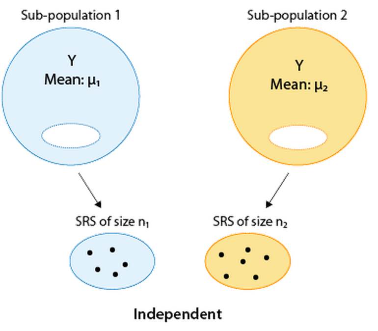
Our goal is comparing μ1 and μ2 (which in practice is done by making inference on the difference μ1 - μ2). The null hypotheses is Ho: μ1 - μ2 = 0
and the alternative hypothesis is one of the following (depending on the context of the problem):
Ha: μ1 - μ2 < 0
Ha: μ1 - μ2 > 0
Ha: μ1 - μ2 ≠ 0The two-sample t-test can be safely used when the samples are independent and at least one of the following two conditions hold: The variable Y is known to have a normal distribution in both populations The two sample sizes are large.
When the sample sizes are not large (and we therefore need to check the normality of Y in both population), what we do in practice is look at the histograms of the two samples and make sure that there are no signs of non-normality such as extreme skewedness and/or outliers.
The test statistic is as follows and has a t distribution when the null hypothesis is true:
P-values are obtained from the output, and conclusions are drawn as usual, comparing the p-value to the significance level alpha. If Ho is rejected, a 95% confidence interval for μ1 - μ2 can be very insightful and can also be used for the two-sided test.
Matched Pairs: Overview (Comparing Two Means—Matched Pairs (Paired t-Test))
We are still in Case C→Q of inference about relationships, where the explanatory variable is categorical and the response variable is quantitative. As we mentioned in the introduction, we introduce three inferential procedures in this case.
So far we have introduced the first procedure—the two-sample t-test that is used when we are comparing two means and the samples are independent. We now move on to the second procedure, where we also compare two means, but the samples are paired or matched. Every observation in one sample is linked with an observation in the other sample. In this case, the samples are dependent.
One of the most common cases where dependent samples occur is when both samples have the same subjects and they are "paired by subject." In other words, each subject is measured twice on the response variable, typically before and then after some kind of treatment/intervention in order to assess its effectiveness.
Example: SAT Prep Class Suppose you want to assess the effectiveness of an SAT prep class. It would make sense to use the matched pairs design and record each sampled student's SAT score before and after the SAT prep classes are attended:
Recall that the two populations represent the two values of the explanatory variable. In this situation, those two values come from a single set of subjects. In other words, both populations really have the same students. However, each population has a different value of the explanatory variable. Those values are: no prep class, prep class.
This, however, is not the only case where the paired design is used. Other cases are when the pairs are "natural pairs," such as siblings, twins, or couples. We will present two examples in this part. The first one will be of the type where each subject is measured twice, and the second one will be a study involving twins.
This section on matched pairs design will be organized very much like the previous section on two independent samples. We will first introduce our leading example, and then present the paired t-test illustrating each step using our example. We will then look at another example, and finally talk about estimation using a confidence interval. As usual, you'll be able to check your understanding along the way, and will learn how to use software to carry out this test.
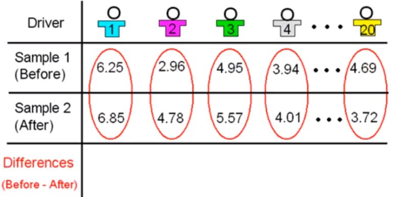
Example: Drunk Drivers Drunk driving is one the main causes of car accidents. Interviews with drunk drivers who were involved in accidents and survived revealed that one of the main problems is that drivers do not realize that they are impaired, thinking "I only had 1-2 drinks ... I am OK to drive." A sample of 20 drivers was chosen, and their reaction times in an obstacle course were measured before and after drinking two beers. The purpose of this study was to check whether drivers are impaired after drinking two beers. Here is a figure summarizing this study:
Comments Note that the categorical explanatory variable here is "drinking 2 beers (Yes/No)", and the quantitative response variable is the reaction time.
Note that by using the matched pairs design in this study (i.e., by measuring each driver twice), the researchers isolated the effect of the two beers on the drivers and eliminated any other confounding factors that might influence the reaction times (such as the driver's experience, age, etc.).
For each driver, the two measurements are the total reaction time before drinking two beers, and after. You can see the data here:
Before After 1 6.25 6.85 2 2.96 4.78 3 4.95 5.57 4 3.94 4.01 5 4.85 5.91 6 4.81 5.34 7 6.60 6.09 8 5.33 5.84 9 5.19 4.19 10 4.88 5.75 11 5.75 6.25 12 5.26 7.23 13 3.16 4.55 14 6.65 6.42 15 5.49 5.25 16 4.05 5.59 17 4.42 3.96 18 4.99 5.93 19 5.01 6.03 20 4.69 3.72
Matched Pairs: Idea Behind the Paired t-test
we have discussed and illustrated cases in which the matched pairs design comes up, and we are now ready to discuss how to carry out the test in this case. We will first present the idea behind the paired t-test, and then go through the four steps in the testing process.
The Paired t-test : Idea The idea behind the paired t-test is to reduce this two-sample situation, where we are comparing two means, to a single sample situation where we are doing inference on a single mean, and then use a simple t-test that we introduced in the previous module. We will first illustrate this idea using our example, and then more generally.
In our example we have 20 drivers and for each one of them we have two measurements: the measurement in sample one, which is the total reaction time before drinking the two beers; and the measurement in sample two, the total reaction time after drinking the two beers.
Since we can view these two samples as twenty pairs of observations, it makes sense to talk about the difference between the two measurements for each driver.
The difference in total reaction time before the two beers minus after the two beers. For example the difference in total reaction time for the first driver is 6.25 - 6.85 which is - 0.6. The difference in total reaction time for the second driver is 2.96 - 4.78 which is - 1.82.
Similarly, we can obtain the difference in total reaction time for each of the drivers and obtain a sample of twenty differences. Note that by obtaining the differences, we reduce our data from two samples to one sample of differences. The paired t test is based on the one sample of differences.
In other words, by reducing the two samples to one sample of differences, we are essentially reducing the problem from a problem where we're comparing two means (i.e., doing inference on \( \mu_1 - \mu_2 \) ):
to a problem where we are making an inference about a single mean — the mean of the differences:
In general, in every matched pairs problem, our data consist of 2 samples which are organized in n pairs:
We reduce the two samples to only one by calculating for each pair the difference between the two observations (in the figure we used \( d_1, d_2, ... , d_n\) to denote the differences).
The paired t-test is based on this one sample of n differences,
and it uses those differences as data for a simple t-test on a single mean — the mean of the differences.
This is the general idea behind the paired t-test; it is nothing more than a regular one-sample t-test for the mean of the differences. We will now go through the 4-step process of the paired t-test.
Matched Pairs: Hypotheses
Step 1: Stating the hypotheses. Recall that in the t-test for a single mean our null hypothesis was: \( H_0: \mu = \mu_0 \) and the alternative was one of \( H_a: \mu < or > or \neq \mu_0 \) . Since the paired t-test is a special case of the one-sample t-test, the hypotheses are the same except that:
Instead of simply μ we use the notation \( \mu_d \) to denote that the parameter of interest is the mean of the differences.
In this course our null value \( \mu_0 \) is always 0 (although technically, it does not have to be).
Therefore, in the paired t-test:
The null hypothesis is always: \( H_0 : \mu_d = 0 \)
and the alternative is one of : \( H_a: \mu_d < 0 (one-sided), H_a: \mu_d > 0 (one-sided), H_a: \mu_d \neq 0 (two-sided) \) depending on the context.
Example: Drunk Driving Recall that in our "Are drivers impaired after drinking two beers?" example, our data was reduced to one sample of differences (one for each driver),
so our problem was reduced to inference about the mean of the differences
As we mentioned, the null hypothesis is: \( H_0 : \mu_d = 0 \) .
The null hypothesis claims that the differences in reaction times are centered at (or around) 0, indicating that drinking two beers has no real impact on reaction times. In other words, drivers are not impaired after drinking two beers.
In order to decide which of the alternatives is appropriate here we have to think about the context of the problem. Recall that we want to check whether drivers are impaired after drinking two beers. Thus, we want to know whether their reaction times are longer after the two beers. Since the differences were calculated before-after, longer reaction times after the beers would translate into negative differences. These differences are: 6.25 - 6.85, 2.96 - 4.78, etc.
Therefore, the appropriate alternative here is: \( H_a : \mu_d < 0 \) indicating that the differences are centered at a negative number.
Question: Many students wonder whether in matched-pairs analysis you should always calculate the differences "response 1 - response 2," or whether it is possible to calculate and do the analysis using the differences "response 2 - response 1."
Answer: Both ways of calculating the differences are fine (as long, of course, as all the differences are calculated the same way). You should pay careful attention to how the differences are calculated, since that will determine the direction of the alternative hypothesis (in the one-sided case). In our example, the differences in reaction times were calculated: before 2 beers - after 2 beers, and therefore in order to test whether drivers are impaired after two beers (i.e., whether their reaction times are longer after drinking two beers) the appropriate hypotheses are:
\( H_0: \mu_d = 0 \text{ v/s } H_a: \mu_d < 0 \)
However, if the differences were calculated: after 2 beers - before 2 beers, the appropriate alternative hypothesis would also change direction, and we would test:
\( H_0: \mu_d = 0 \text{ v/s } H_a: \mu_d > 0 \)
Comment Recall that originally, the following figure represented our problem:
Later, we reduced the problem to inference about a single mean, the mean of the differences:
Some students find it helpful to know that it turns out that \( \mu_d = \mu_1 - \mu_2 \). In other words, the difference between the means \( \mu_1 - \mu_2 \) in the first representation is the same as the mean of the differences, \( \mu_d \) ,in the second one. Some students find it easier to first think about the hypotheses in terms of \( \mu_1 - \mu_2 \) (as we did in the two-sample case) and then represent it in terms of \( \mu_d \).
In our example, since we want to test whether the reaction times in population 1 are shorter, we are testing \( H_0 : \mu_1 - \mu_2 = 0 \text{ v/s } H_a: \mu_1 - \mu_2 < 0 \), which in the matched pairs design notation is translated to \( H_0: \mu_d = 0 \text{ v/s } H_a: \mu_d < 0 \) .
Example Suppose the effectiveness of a low-carb diet is studied with a matched pairs design, recording each participant's weight before and after dieting. What would be the appropriate hypotheses in this case?
As before, \( \mu_d \) is the mean of the differences (weight before diet)-(weight after diet). In this case, if the diet is effective and participants' weight after the diet was indeed lower, we would expect the differences to be positive, and therefore the appropriate hypotheses in this case are: \( H_0: \mu_d = 0 \text{ v/s } H_a: \mu_d > 0 \)
- Explanation :
Indeed, if the drug is effective, we would expect the participants' cholesterol levels to be lower after taking it for 6 weeks. This means that we expect the differences (level before - level after) to be positive, and therefore the appropriate hypotheses in this case are (Ho: μd = 0) and (Ha: μd > 0).
- Explanation :
Indeed this is not a matched pairs situation. Since two (different) random samples of secretaries were chosen, these two samples are independent, and not matched.
- Explanation :
Indeed, since we would like to test whether the typing speeds differ, the appropriate hypotheses are: (Ho: μd = 0) and (Ha: μd ≠ 0).
Matched Pairs: Conditions and Paired t-test
Step 2: Checking Conditions and Calculating the Test Statistic
The paired t-test, as a special case of a one-sample t-test, can be safely used as long as:
The sample of differences is random (or at least can be considered so in context).
We are in one of the three situations marked with a green check mark in the following table
In other words, in order to use the paired t-test safely, the differences should vary normally unless the sample size is large, in which case it is safe to use the paired t-test regardless of whether the differences vary normally or not. As we indicated in the figure above (and have seen many times already), in practice, normality is checked by looking at the histogram of differences and as long as no clear violation of normality (such as extreme skewness and/or outliers) is apparent, normality is assumed. Assuming that the we can safely use the paired t-test, the data are summarized by a test statistic: \( t = \frac{\overline{x_d} - 0}{\frac{s_d}{\sqrt{n}}} \)
where \( \overline{x_d} \) is the sample mean of the differences, and \( s_d \) is the sample standard deviation of the differences. This is the test statistic we've developed for the one sample t-test (with \( \mu_0 = 0 \) ), and has the same conceptual interpretation; it measures (in standard errors) how far our data are (represented by the average of the differences) from the null hypothesis (represented by the null value, 0).
Example Let's first check whether we can safely proceed with the paired t-test, by checking the two conditions.
The sample of drivers was chosen at random.
The sample size is not large enough (n = 20), so in order to proceed, we need to look at the histogram of the differences and make sure there is no evidence that the normality assumption is not met. Here is the histogram:
There is no evidence of violation of the normality assumption (on the contrary, the histogram looks quite normal). Also note that the vast majority of the differences are negative (i.e., the total reaction times for most of the drivers are larger after the two beers), suggesting that the data provide evidence against the null hypothesis.
The question (which the p-value will answer) is whether these data provide strong enough evidence or not. We can safely proceed to calculate the test statistic (which in practice we leave to the software to calculate for us).
Here is the output of the paired t-test for our example:
According to the output, the test statistic is -2.58, indicating that the data (represented by the sample mean of the differences) are 2.58 standard errors below the null hypothesis (represented by the null value, 0). Note in the output, that beyond the test statistic itself, we also highlighted the part of the output that provides the ingredients needed in order to calculate it: \( n = 20; \overline{x_d} = -0.5015, s_d = 0.8686\) . Indeed \( \frac{-0.5015}{\frac{0.8686}{\sqrt{20}}} = -2.58 \).
Matched Pairs: Finding the p-value
Step 3: Finding the p-value As a special case of the one-sample t-test, the null distribution of the paired t-test statistic is a t distribution (with n - 1 degrees of freedom), which is the distribution under which the p-values are calculated. We will let the software find the p-value for us, and in this case, Excel gives us a p-value of 0.009.
The small p-value tells us that there is very little chance of getting data like those observed (or even more extreme) if the null hypothesis were true. More specifically, there is less than a 1% chance (0.009=.9%) of obtaining a test statistic of -2.58 (or lower), assuming that 2 beers have no impact on reaction times.
Step 4: Conclusion in Context As usual, we draw our conclusion based on the p-value. If the p-value is small, there is a significant difference between what was observed in the sample and what was claimed in Ho, so we reject Ho and conclude that the categorical explanatory variable does affect the quantitative response variable as specified in Ha. If the p-value is not small, we do not have enough statistical evidence to reject Ho. In particular, if a cutoff probability, α (significance level), is specified, we reject Ho if the p-value is less than α. Otherwise, we do not reject Ho.
In our example, the p-value is 0.009, indicating that the data provide enough evidence to reject Ho and conclude that drinking two beers does slow the reaction times of drivers, and thus that drivers are impaired after drinking two beers.
Comment It is very important to pay attention to whether the two-sample t-test or the paired t-test is appropriate. In other words, being aware of the study design is extremely important. Consider our example. If we had not "caught" that this is a matched pairs design, and had analyzed the data as if the two samples were independent using the two-sample t-test, we would have obtained a p-value of 0.057.
Note that using this (wrong) method to analyze the data, and a significance level of 0.05, we would conclude that the data do not provide enough evidence for us to conclude that drivers are impaired after drinking two beers. This is an example of how using the wrong statistical method can lead you to wrong conclusions, which in this context can have very serious implications.
Matched Pairs: Example
The "driving after having 2 beers" example is a case in which observations are paired by subject. In other words, both samples have the same subject, so that each subject is measured twice. Typically, as in our example, one of the measurements occurs before a treatment/intervention (2 beers in our case), and the other measurement after the treatment/intervention. Our next example is another typical type of study where the matched pairs design is used—it is a study involving twins.
Example Researchers have long been interested in the extent to which intelligence, as measured by IQ score, is affected by "nurture" as opposed to "nature": that is, are people's IQ scores mainly a result of their upbringing and environment, or are they mainly an inherited trait? A study was designed to measure the effect of home environment on intelligence, or more specifically, the study was designed to address the question: "Are there significant differences in IQ scores between people who were raised by their birth parents, and those who were raised by someone else?"
In order to be able to answer this question, the researchers needed to get two groups of subjects (one from the population of people who were raised by their birth parents, and one from the population of people who were raised by someone else) who are as similar as possible in all other respects. In particular, since genetic differences may also affect intelligence, the researchers wanted to control for this confounding factor.
We know from our discussion on study design (in the Producing Data unit of the course) that one way to (at least theoretically) control for all confounding factors is randomization—randomizing subjects to the different treatment groups. In this case, however, this is not possible. This is an observational study; you cannot randomize children to either be raised by their birth parents or to be raised by someone else. How else can we eliminate the genetics factor? We can conduct a "twin study."
Because identical twins are genetically the same, a good design for obtaining information to answer this question would be to compare IQ scores for identical twins, one of whom is raised by birth parents and the other by someone else. Such a design (matched pairs) is an excellent way of making a comparison between individuals who only differ with respect to the explanatory variable of interest (upbringing) but are as alike as they can possibly be in all other important aspects (inborn intelligence). Identical twins raised apart were studied by Susan Farber, who published her studies in the book "Identical Twins Reared Apart" (1981, Basic Books). In this problem, we are going to use the data that appear in Farber's book in table E6, of the IQ scores of 32 pairs of identical twins who were reared apart.
Here is a figure that will help you understand this study:
Here are the important things to note in the figure:
We are essentially comparing the mean IQ scores in two populations that are defined by our (two-valued categorical) explanatory variable — upbringing (X), whose two values are: raised by birth parents, raised by someone else.
This is a matched pairs design (as opposed to a two independent samples design), since each observation in one sample is linked (matched) with an observation in the second sample. The observations are paired by twins.
Here is the data set:
Twin 1 Twin 2 1 113 109 2 94 100 3 99 86 4 77 80 5 81 95 6 91 106 7 111 117 8 104 107 9 85 85 10 66 84 11 111 125 12 51 66 13 109 108 14 122 121 15 97 98 16 82 94 17 100 88 18 100 104 19 93 84 20 99 95 21 109 98 22 95 100 23 75 86 24 104 103 25 73 78 26 88 99 27 92 111 28 108 110 29 88 83 30 90 82 31 79 76 32 97 98 Each of the 32 rows represents one pair of twins. Keeping the notation that we used above, twin 1 is the twin that was raised by his/her birth parents, and twin 2 is the twin that was raised by someone else. Let's carry out the analysis.
Stating the hypotheses.
Recall that in matched pairs, we reduce the data from two samples to one sample of differences:
-
and we state our hypotheses in terms of the mean of the differences, \( \mu_d \).
Since we would like to test whether there are differences in IQ scores between people who were raised by their birth parents and those who weren't, we are carrying out the two-sided test:
\( H_0 = \mu_d = 0, H_a: \mu_d \neq 0 \)
Comment:
Again, some students find it easier to first think about the hypotheses in terms of μ1 and μ2, and then write them in terms of \( \mu_d \). In this case, since we are testing for differences between the two populations, the hypotheses will be:
\( H_0: \mu_1 - \mu_2 = 0, H_a: \mu_1 - \mu_2 \neq 0 \)
and since \( \mu_d = \mu_1 - \mu_2 \) we get back to the hypotheses above.Checking conditions and summarizing the data with a test statistic.
Is it safe to use the paired t-test in this case?
Clearly, the samples of twins are not random samples from the two populations. However, in this context, they can be considered as random, assuming that there is nothing special about the IQ of a person just because he/she has an identical twin.
The sample size here is n = 32. Even though it's the case that if we use the n > 30 rule of thumb our sample can be considered large, it is sort of a borderline case, so just to be on the safe side, we should look at the histogram of the differences just to make sure that we do not see anything extreme. (Comment: Looking at the histogram of differences in every case is useful even if the sample is very large, just in order to get a sense of the data. Recall: "Always look at the data.")
The data don't reveal anything that we should be worried about (like very extreme skewness or outliers), so we can safely proceed. Looking at the histogram, we note that most of the differences are negative, indicating that in most of the 32 pairs of twins, twin 2 (raised by someone else) has a higher IQ.
From this point we rely on statistical software, and find that:
t-value = -1.85
p-value = 0.074
Our test statistic is -1.85. Our data (represented by the average of the differences) are 1.85 standard errors below the null hypothesis (represented by the null value 0).Finding the p-value.
The p-value is 0.074, indicating that there is a 7.4% chance of obtaining data like those observed (or even more extreme) assuming that Ho is true (i.e., assuming that there are no significant differences in IQ scores between people who were raised by their natural parents and those who weren't).
Making conclusions.
Using the conventional significance level (cut-off probability) of 0.05, our p-value is not small enough, and we therefore cannot reject Ho. In other words, our data do not provide enough evidence to conclude that whether a person was raised by his/her natural parents has an impact on the person's intelligence (as measured by IQ scores).
Comment This means that if, based on prior knowledge, prior research, or just a hunch, we had wanted to test the hypothesis that the IQ level of people raised by their birth parents is lower, on average, than the IQ level of people who were raised by someone else, we would have rejected Ho and accepted that hypothesis (at the 0.05 significance level, since 0.037 < 0.05).
It should be stressed, though, that one should set the hypotheses before looking at the data. It would be ethically wrong to look at the histogram of differences, note that most of the differences are negative, and then decide to carry out the one-sided test that the data seem to support. This is known as "data snooping," and is considered to be a very bad statistical practice.
- Explanation :
Indeed, the p-value of the one-sided test is half the p-value of the two-sided test.