Scenario: Gosset's Seed Plot Data
William S. Gosset was employed by the Guinness brewing company of Dublin. Sample sizes available for experimentation in brewing were necessarily small, and new techniques for handling the resulting data were needed. Gosset consulted Karl Pearson (1857-1936) of University College in London, who told him that the current state of knowledge was unsatisfactory. Gosset undertook a course of study under Pearson and the outcome of his study was perhaps the most famous paper in statistical literature, "The Probable Error of a Mean" (1908), which introduced the t distribution.
Since Gosset was contractually bound by Guinness, he published under a pseudonym, "Student," hence the t distribution is often referred to as Student's t distribution.
As an example to illustrate his analysis, Gosset reported in his paper on the results of seeding 11 different plots of land with two different types of seed: regular and kiln-dried. There is reason to believe that drying seeds before planting will increase plant yield. Since different plots of soil may be naturally more fertile, this confounding variable was eliminated by using the matched pairs design and planting both types of seed in all 11 plots.
The resulting data (corn yield in pounds per acre) are as follows:
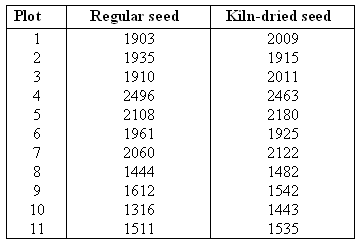
We are going to use these data to test the hypothesis that kiln-dried seed yields more corn than regular seed. Here is a figure that summarizes this problem:
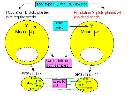
Because of the nature of the experimental design (matched pairs), we are testing the difference in yield.
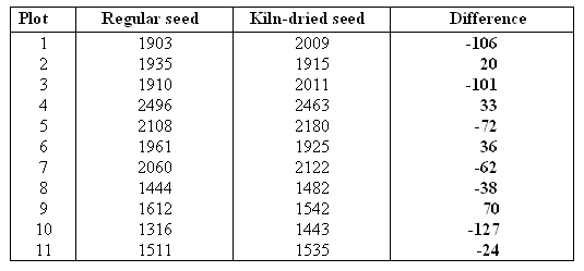
Note that the differences were calculated: regular - kiln-dried.
State the appropriate hypotheses that are being tested here. Be sure to define the parameter that you are using.
Let ռsub>d be the mean of the yield difference "regular - kiln-dried" in a plot. Since we want to test the hypothesis that kiln-dried seed yields more corn than regular seed, the appropriate hypotheses are: \( H_0: \mu_d = 0 H_a: \mu_d < 0 \)
We created a histogram and boxplot of the differences data below.


Are the conditions that allow you to safely use the paired t-test satisfied?
Let's check the conditions: (i) Even though the problem does not state it specifically, we can assume that Gosset "knew what he was doing" and the plots were chosen at random.
(ii) The sample size is quite small (n = 11), so we need to make sure that the data (differences) do not display any extreme departure from the normality assumption. Typically we look at a histogram.
Comment: some prefer to look at a boxplot of the data, since outliers are clearly marked, and skewness is apparent by the location of the middle line inside the box (which represents the location of the median relative to the quartiles). We recommend looking at the histogram (as we did previously) or at both graphs.
Both graphs show us that the data does not display any departure from the normality assumption in the form of extreme skewness and/or outliers.
Note that 1) with such a small sample size of n = 11 we cannot really expect to see a normal shape in the histogram; so as long as we don't see anything that is extremely "non-normal," we're fine.
2) The boxplot shows us that no observation was classified as an outlier, and that there is no extreme skewness, since the median - the line inside the box - is roughly in the middle of the box). In summary, we can safely proceed with the paired t-test.
Based on the visual displays, does it seem like there is some evidence in the data in favor of the alternative hypothesis? Explain.
We notice that most of the differences (7 out of 11) are negative, indicating that in 7 of the 11 plots, the dry seeds produced more corn yield. This is evidence in favor of the alternative hypothesis, but the evidence is not overwhelming, so it is hard to say whether this is strong enough evidence to reject the null hypothesis in favor of the alternative
We conducted the paired t-test and found the t statistic to be -1.69 with a p-value of 0.0609. What conclusions would you draw?
The test statistic is -1.69 and the p-value is 0.061, indicating that there is a 6.1% chance of obtaining data like those observed (or even more extremely in favor of the alternative hypothesis) had there really been no difference between regular and kiln-dried seeds (as the null hypothesis claims).
Even though the p-value is quite small, it is not small enough if we use a significance level (cut-off probability) of 0.05. This means that even though the data show some evidence against the null hypothesis, it isn't quite strong enough to reject it.
We therefore conclude that the data do not provide enough evidence that kiln-dried seeds yield more corn than regular seeds. Comment: While it is true that at the 0.05 significance level, our p-value is not small enough to reject Ho, it is "almost small enough."
In other words, this is sort of a "borderline case" where personal interpretation and/or judgment is in order.
You can stick to the 0.05 cut-off as we did above in our conclusion, but you might decide that 0.061 is small enough for you, and that the evidence that the data provide is strong enough for you to believe that indeed kiln-dried seeds yield more corn.
This is the beauty of statistics ... there is no "black or white," and there is a lot of room for personal interpretation.
Matched Pairs: Confidence Interval
Confidence Interval for \( \mu_d \) (Paired t Confidence Interval) So far we've discussed the paired t-test, which checks whether there is enough evidence stored in the data to reject the claim that \( \mu_d = 0 \) in favor of one of the three possible alternatives.
If we would like to estimate \( \mu_d \) , the mean of the differences (response 1 - response 2), we can use the natural point estimate, \( \overline{x_d} \), the sample mean of the differences, or preferably, use a 95% confidence interval, which will provide us with a set of plausible values for \( \mu_d \).
In particular, if the test has rejected \( H_0 : \mu_d = 0 \), a confidence interval for \( \mu_d \) can be insightful, since it quantifies the effect that the categorical explanatory variable has on the response variable.
Comment: We will not go into the formula and calculation of the confidence interval, but rather ask our statistical software to do it for us, and focus on interpretation.
Example Recall our leading example about whether drivers are impaired after having two beers:
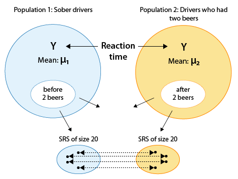 which is reduced to inference about a single mean, the mean of the differences (before - after):
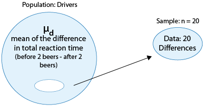
The p-value of our test, \( H_0 : \mu_d = 0 \) vs. \( H_0 : \mu_d < 0 \) was .009, and we therefore rejected Ho and concluded that the mean difference in total reaction time (before beer - after beer) was negative, or in other words, that drivers are impaired after having two beers. As a follow-up to this conclusion, it would be interesting to quantify the effect that two beers have on the driver, using the 95% confidence interval for \( \mu_d \).
Using statistical software, we find that the 95% confidence interval for \( \mu_d \), the mean of the differences (before - after), is roughly (-0.9, -0.1).
We can therefore say with 95% confidence that drinking two beers increases the total reaction time of the driver by between 0.1 and 0.9 of a second.
Comment
As we've seen in previous tests, as well as in the matched pairs case, the 95% confidence interval for \( \mu_d \) can be used for testing in the two-sided case \( H_0 : \mu_d = 0 \text{vs.} H_a : \mu_d \neq 0 \):
If the null value, 0, falls outside the confidence interval, Ho is rejected.
If the null value, 0, falls inside the confidence interval, Ho is not rejected.
Example : Let's go back to our twin study example, where we found a 95% confidence interval for of (-6.11322, 0.30072) and a p-value of 0.074.
We used the fact that the p-value is 0.074 to conclude that Ho can not be rejected (at the 0.05 significance level), and that whether or not a person was raised by his or her birth parents doesn't necessarily have an effect on intelligence (as measured by IQ scores). The last comment tells us that we can also use the confidence interval to reach the same conclusion, since 0 falls inside the confidence interval for \( \mu_d \). In other words, since 0 is a plausible value for \( \mu_d \) we cannot reject Ho which claims that \( \mu_d = 0 \).
Scenario: Typing Speed for Different Word Processors A publishing company wanted to test whether typing speed differs when using word processor A or word processor B. A random sample of 25 typists was selected and the typing speeds (in words per minute) were recorded for each secretary when using word processor A and then when using word processor B. (Which word processor was used first was determined for each typist by a coin flip).
Based on the collected data, a 95% confidence interval for \( \mu_d \), the mean difference (word processor A - word processor B) was found to be (2.5, 7.8).
The appropriate hypotheses for testing whether the typing speeds differ when using word processor A or word processor B is the two-sided test:
\( H_0: \mu_d = 0, H_a: \mu_d \neq 0 \)
Solved Questions
Q. Based on this confidence interval for \( \mu_d \), what would be your conclusion (at the 0.05 significance level)? Explain.
Since 0 (our null value) falls outside the 95% confidence interval, we can reject Ho (at the 0.05 significance level), and conclude that the typing speeds differ when using processor A or B.
Q. Interpret the 95% confidence interval in context. Make sure that your interpretation quantifies the effect that the type of word processor used (the explanatory variable, X) has on the typing speed (the response variable, Y).
We are 95% confident that on average, typists type between 2.5 and 7.8 more words per minute when using word processor A.
Matched Pairs: Summary
The paired t-test is used to compare two population means when the two samples (drawn from the two populations) are dependent in the sense that every observation in one sample can be linked to an observation in the other sample. Such a design is called "matched pairs."

The most common case in which the matched pairs design is used is when the same subjects are measured twice, usually before and then after some kind of treatment and/or intervention. Another classic case are studies involving twins.
The idea behind the paired t-test is to reduce the data from two samples to just one sample of the differences, and use these observed differences as data for inference about a single mean - the mean of the differences, \( \mu_d \).

The paired t-test is therefore simply a one-sample t-test for the mean of the differences \( \mu_d \), where the null value is 0. The null hypothesis is therefore: Ho: \( \mu_d \) = 0
and the alternative hypothesis is one of the following (depending on the context of the problem):
Ha: \( \mu_d \) < 0
Ha: \( \mu_d \) > 0
Ha: \( \mu_d \neq \) 0The paired t-test can be safely used when one of the following two conditions hold:
The differences have a normal distribution.
The sample size of differences is large.
When the sample size of difference is not large (and we therefore need to check the normality of the differences), what we do in practice is look at the histograms of the differences and make sure that there are no signs of non-normality like extreme skewedness and/or outliers.
The test statistic is as follows and has a t distribution when the null hypothesis is true:

P-values are obtained from the output, and conclusions are drawn as usual, comparing the p-value to the significance level alpha.
If Ho is rejected, a 95% confidence interval for \( \mu_d \) can be very insightful and can also be used for the two-sided test.
Comparing More Than Two Means - ANOVA: Overview
In this part, we continue to handle situations involving one categorical explanatory variable and one quantitative response variable, which is case C → Q in our role/type classification table:

So far we have discussed the two samples and matched pairs designs, in which the categorical explanatory variable is two-valued. As we saw, in these cases, examining the relationship between the explanatory and the response variables amounts to comparing the mean of the response variable (Y) in two populations, which are defined by the two values of the explanatory variable (X). The difference between the two samples and matched pairs designs is that in the former, the two samples are independent, and in the latter, the samples are dependent.
We are now moving on to cases in which the categorical explanatory variable takes more than two values. Here, as in the two-valued case, making inferences about the relationship between the explanatory (X) and the response (Y) variables amounts to comparing the means of the response variable in the populations defined by the values of the explanatory variable, where the number of means we are comparing depends, of course, on the number of values of X. Unlike the two-valued case, where we looked at two sub-cases (1) when the samples are independent (two samples design) and (2) when the samples are dependent (matched pairs design, here, we are just going to discuss the case where the samples are independent. In other words, we are just going to extend the two samples design to more than two independent samples.

Comment The extension of the matched pairs design to more than two dependent samples is called "Repeated Measures" and is beyond the scope of this course.
The inferential method for comparing more than two means that we will introduce in this part is called Analysis Of Variance (abbreviated as ANOVA), and the test associated with this method is called the ANOVA F-test. The structure of this part will be very similar to that of the previous two. We will first present our leading example, and then introduce the ANOVA F-test by going through its 4 steps, illustrating each one using the example. (It will become clear as we explain the idea behind the test where the name "Analysis of Variance" comes from.) We will then present another complete example, and conclude with some comments about possible follow-ups to the test. As usual, you'll have activities along the way to check your understanding, and learn how to use software to carry out the test.
Example Is "academic frustration" related to major?
A college dean believes that students with different majors may experience different levels of academic frustration. Random samples of size 35 of Business, English, Mathematics, and Psychology majors are asked to rate their level of academic frustration on a scale of 1 (lowest) to 20 (highest).

The figure highlights what we have already mentioned: examining the relationship between major (X) and frustration level (Y) amounts to comparing the mean frustration levels \( \mu_1, \mu_2, \mu_3, \mu_4 \) among the four majors defined by X. Also, the figure reminds us that we are dealing with a case where the samples are independent.
Comment There are two ways to record data in the ANOVA setting:
Unstacked: One column for each of the four majors, with each column listing the frustration levels reported by all sampled students in that major:
Business English Math Psychology 11 11 9 11 6 9 16 19 6 14 11 13 etc. Stacked: one column for all the frustration levels, and next to it a column to keep track of which major a student is in:
Frustration(Y) Major(X) 9 Business 2 Business 9 Business 10 English 11 Psychology 13 English 13 Psychology 12 Math etc. The "unstacked" format helps us to look at the four groups separately, while the "stacked" format helps us remember that there are, in fact, two variables involved: frustration level (the quantitative response variable) and major (the categorical explanatory variable).
Here are the first 50 cases that were loaded into a statistics software package:
Business English Mathematics Psychology Frustration Score Major 1 11 11 9 11 11 Business 2 6 9 16 19 6 Business 3 6 14 11 13 6 Business 4 4 13 11 10 4 Business 5 6 9 12 14 6 Business 6 9 12 17 10 9 Business 7 8 10 12 13 8 Business 8 3 12 14 14 3 Business 9 11 9 20 15 11 Business 10 12 11 12 17 12 Business 11 7 15 14 17 7 Business 12 5 13 15 14 5 Business 13 2 10 14 13 2 Business 14 11 10 14 9 12 Business 15 13 15 12 19 13 Business 16 9 11 15 17 9 Business 17 9 13 14 17 9 Business 18 9 9 12 11 9 Business 19 5 15 14 13 5 Business 20 8 17 14 19 8 Business 21 6 12 14 8 6 Business 22 3 10 14 20 3 Business 23 5 12 9 15 5 Business 24 10 9 14 14 10 Business 25 9 8 15 15 9 Business 26 6 14 12 15 6 Business 27 4 13 17 9 4 Business 28 8 13 13 16 8 Business 29 10 13 13 16 10 Business 30 2 11 11 11 2 Business 31 8 12 15 14 8 Business 32 4 11 14 13 4 Business 33 9 13 9 11 9 Business 34 9 12 15 16 9 Business 35 9 11 16 13 9 Business 36 NA NA NA NA 11 English 37 NA NA NA NA 9 English 38 NA NA NA NA 14 English 39 NA NA NA NA 13 English 40 NA NA NA NA 9 English 41 NA NA NA NA 12 English 42 NA NA NA NA 10 English 43 NA NA NA NA 12 English 44 NA NA NA NA 9 English 45 NA NA NA NA 11 English 46 NA NA NA NA 15 English 47 NA NA NA NA 13 English 48 NA NA NA NA 10 English 49 NA NA NA NA 10 English 50 NA NA NA NA 15 English Note that in the first 4 columns, the data are in unstacked format, and in the next two columns the data are stacked.
The ANOVA F-test: Hypotheses
Now that we understand in what kind of situations ANOVA is used, we are ready to learn how it works, or more specifically, what the idea is behind comparing more than two means. As we mentioned earlier, the test that we will present is called the ANOVA F-test, and as you'll see, this test is different in two ways from all the tests we have presented so far:
Unlike the previous tests, where we had three possible alternative hypotheses to choose from (depending on the context of the problem), in the ANOVA F-test there is only one alternative, which actually makes life simpler.
The test statistic will not have the same structure as the test statistics we've seen so far. In other words, it will not have the form: \( \frac{\text{sample statistic - null value}}{\text{standard error}} \), but a different structure that captures the essence of the F-test, and clarifies where the name "analysis of variance" is coming from.
Step 1: Stating the Hypotheses
The null hypothesis claims that there is no relationship between X and Y. Since the relationship is examined by comparing \( \mu_1, \mu_2, \mu_3, .. , \mu_k \), the means of Y in the populations defined by the values of X, no relationship would mean that all the means are equal. Therefore the null hypothesis of the F-test is: \( H_0: \mu_1 = \mu_2 = \mu_3 = .. = \mu_k \)
As we mentioned earlier, here we have just one alternative hypothesis, which claims that there is a relationship between X and Y. In terms of the means \( \mu_1, \mu_2, \mu_3, .. , \mu_k \), it simply says the opposite of the alternative, that not all the means are equal, and we simply write: \( H_a : \text{not all the \mu are equal } \).
Example : Recall our "Is academic frustration related to major?" example:

The correct hypotheses for our example are: \( H_0: \mu_1 = \mu_2 = \mu_3 = \mu_4, H_a: \text{not all the \mu's are equal} \)
Note that there are many ways for \( \mu_1 , \mu_2 , \mu_3 , \mu_4 \) not to be all equal, and \( \mu_1 \neq \mu_2 \neq \mu_3 \neq \mu_4 \) is just one of them. Another way could be \( \mu_1 = \mu_2 = \mu_3 \neq \mu_4 \) or \( \mu_1 = \mu_2 \neq \mu_3 = \mu_4 \). The alternative of the ANOVA F-test simply states that not all of the means are equal, and is not specific about the way in which they are different.
- Explanation :
Indeed, while the null hypothesis is correct, the alternative hypothesis isn't. We recommend that you read our explanation that follows even if you think you understand why the alternative hypothesis is wrong.