• Let's think about how we would go about testing whether the population means \( \mu_1, \mu_2, \mu_3, \mu_4 \) are equal. It seems as if the best we could do is to calculate their point estimates - the sample mean in each of our 4 samples (denote them by \( \overline{y_1}, \overline{y_2}, \overline{y_3}, \overline{y_4} \) ),




• 




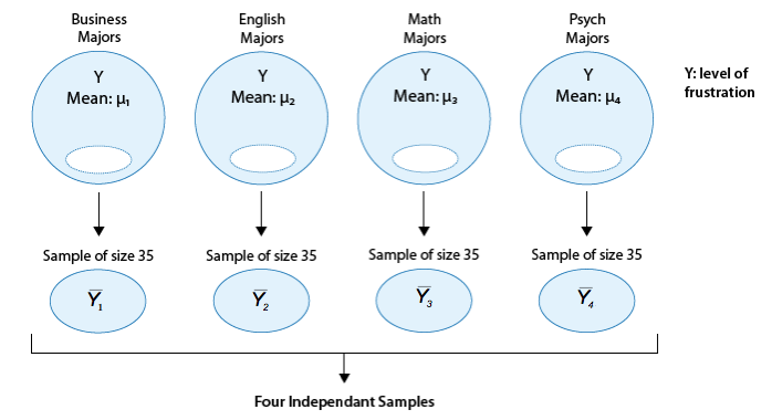
• and see how far apart these sample means are, or in other words, measure the variation between the sample means. If we find that the four sample means are not all close together, we'll say that we have evidence against Ho, and otherwise, if they are close together, we'll say that we do not have evidence against Ho. This seems quite simple, but is this enough? Let's see.




• It turns out that:




1. * The sample mean frustration score of the 35 business majors is: \( \overline{y_1} = 7.3 \)




2. * The sample mean frustration score of the 35 English majors is: \( \overline{y_2} = 11.8 \)




3. * The sample mean frustration score of the 35 math majors is: \( \overline{y_3} = 13.2 \)




4. * The sample mean frustration score of the 35 psychology majors is: \( \overline{y_4} = 14.0 \)




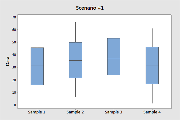
• Below we present two possible scenarios for our example. In both cases, we construct side-by-side boxplots for four groups of frustration levels that have the same variation among their means. Thus, Scenario #1 and Scenario #2 both show data for four groups with the sample means 7.3, 11.8, 13.2, and 14.0 (indicated with red marks).




• 

  Q.

  Look carefully at the graphs of both scenarios. For which of the two scenarios would you be willing to believe that samples have been taken from four groups which have the same population means?

  Scenario 1
  Scenario 2
  
  
  View Answer
  
  

  1. Explanation :

     Your intuition is right. Read on to understand what's going on here.

  
  
  




• The important difference between the two scenarios is that the first represents data with a large amount of variation within each of the four groups; the second represents data with a small amount of variation within each of the four groups.




• Scenario 1, because of the large amount of spread within the groups, shows boxplots with plenty of overlap. One could imagine the data arising from 4 random samples taken from 4 populations, all having the same mean of about 11 or 12. The first group of values may have been a bit on the low side, and the other three a bit on the high side, but such differences could conceivably have come about by chance. This would be the case if the null hypothesis, claiming equal population means, were true. Scenario 2, because of the small amount of spread within the groups, shows boxplots with very little overlap. It would be very hard to believe that we are sampling from four groups that have equal population means. This would be the case if the null hypothesis, claiming equal population means, were false.




• Thus, in the language of hypothesis tests, we would say that if the data were configured as they are in scenario 1, we would not reject the null hypothesis that population mean frustration levels were equal for the four majors. If the data were configured as they are in scenario 2, we would reject the null hypothesis, and we would conclude that mean frustration levels differ, depending on major.




• Let's summarize what we learned from this. The question we need to answer is: Are the differences among the sample means (\( \overline{Y} \)'s) due to true differences among the \( \mu \)'s (alternative hypothesis), or merely due to sampling variability (null hypothesis)?




• In order to answer this question using our data, we obviously need to look at the variation among the sample means, but this alone is not enough. We need to look at the variation among the sample means relative to the variation within the groups. In other words, we need to look at the quantity:




• which measures to what extent the difference among the sampled groups' means dominates over the usual variation within sampled groups (which reflects differences in individuals that are typical in random samples).




• When the variation within groups is large (like in scenario 1), the variation (differences) among the sample means could become negligible and the data provide very little evidence against Ho. When the variation within groups is small (like in scenario 2), the variation among the sample means dominates over it, and the data have stronger evidence against Ho.




• Looking at this ratio of variations is the idea behind the comparing more than two means; hence the name analysis of variance (ANOVA).




• Now that we understand the idea behind the ANOVA F-test, let's move on to step 2. We'll start by talking about the test statistic, since it will be a natural continuation of what we've just discussed, and then move on to talk about the conditions under which the ANOVA F-test can be used. In practice, however, the conditions need to be checked first, as we did before.

• Step 2: Checking Conditions and Finding the Test Statistic The test statistic of the ANOVA F-test, called the F statistic, has the form




• 




• As we mentioned earlier, it has a different structure from all the test statistics we've looked at so far; however, it is similar in that it is still a measure of the evidence against Ho. The larger F is (which happens when the denominator, the variation within groups, is small relative to the numerator, the variation among the sample means), the more evidence we have against Ho.




• Consider the following generic situation:




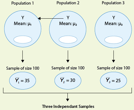
• where we're testing: \( H_0: \mu_1 = \mu_2 = \mu_3, H_a: \text{not all the μ's are equal} \)




• The following are two possible scenarios of the data (note in both scenarios the sample means are 25, 30, and 3




• 




• 

View Answer



View Answer


View Answer


View Answer


View Answer


View Answer


View Answer


View Answer

• Suppose that we would like to compare four populations (for example, four races/ethnicities or four age groups) with respect to a certain psychological test score. More specifically we would like to test: \( H_0 : \mu_1 = \mu_2 = \mu_3 = \mu_4 \)




• H_a : Not all the μ's are equal




• Where: \( \mu_1 \) is the mean test score in population 1 \( \mu_2 \) is the mean test score in population 2 \( \mu_3 \) is the mean test score in population 3 \( \mu_4 \) is the mean test score in population 4




• We take a random sample from each population and use these four independent samples in order to carry out the test.




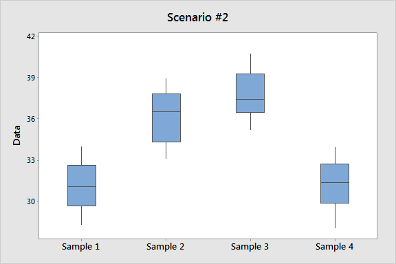
• The following are two possible scenarios for the data:




• 




• 




• 




• 




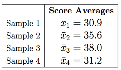
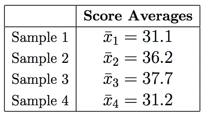
• Note that in both scenarios, the score averages of the four samples are very similar.




• Comments




• The focus here is for you to understand the idea behind this test statistic. We are not going to go into any of the details about how the two variations are measured. This will be included in an extension module to this course in the future. We will rely on software output to obtain the F-statistic.




• This test is called the ANOVA F-test. So far, we have explained the ANOVA part of the name. Based on the previous tests we introduced, it should not be surprising that the "F-test" part comes from the fact that the null distribution of the test statistic, under which the p-values are calculated, is called an F-distribution. We will say very little about the F-distribution in this course, which will essentially be limited to this comment and the next one.




• It is fairly straightforward to decide if a z-statistic is large. Even without tables, we should realize by now that a z-statistic of 0.8 is not especially large, whereas a z-statistic of 2.5 is large. In the case of the t-statistic, it is less straightforward, because there is a different t-distribution for every sample size n (and degrees of freedom n - 1). However, the fact that a t-distribution with a large number of degrees of freedom is very close to the Z (standard normal) distribution can help to assess the magnitude of the t-test statistic.




• When the size of the F-statistic must be assessed, the task is even more complicated, because there is a different F-distribution for every combination of the number of groups we are comparing and the total sample size. We will nevertheless say that for most situations, an F-statistic greater than 4 would be considered rather large, but tables or software are needed to get a truly accurate assessment.

View Answer



View Answer



View Answer

• 




• Here is the statistics software output for the ANOVA F-test. In particular, note that the F-statistic is 46.60 which is very large, indicating that the data provide a lot of evidence against Ho . (we can also see that the p-value is so small that it is essentially 0, which supports that conclusion as well).




• Let's move on to talk about the conditions under which we can safely use the ANOVA F-test, where the first two conditions are very similar to ones we've seen before, but there is a new third condition. It is safe to use the ANOVA procedure when the following conditions hold:




• The samples drawn from each of the populations we're comparing are independent.




• The response variable varies normally within each of the populations we're comparing. As you already know, in practice this is done by looking at the histograms of the samples and making sure that there is no evidence of extreme departure from normality in the form of extreme skewness and outliers. Another possibility is to look at side-by-side boxplots of the data, and add histograms if a more detailed view is necessary. For large sample sizes, we don't really need to worry about normality, although it is always a good idea to look at the data.




• The populations all have the same standard deviation. The best we can do to check this condition is to find the sample standard deviations of our samples and check whether they are "close." A common rule of thumb is to check whether the ratio between the largest sample standard deviation and the smallest is less than 2. If that's the case, this condition is considered to be satisfied.

• In our example all the conditions are satisfied:




• All the samples were chosen randomly, and are therefore independent.




• The sample sizes are large enough (n = 35) that we really don't have to worry about the normality; however, let's look at the data using side-by-side boxplots, just to get a sense of it:




• 




• You'll recognize this plot as Scenario 2 from earlier. The data suggest that the frustration level of the business students is generally lower than students from the other three majors. The ANOVA F-test will tell us whether these differences are significant.




• In order to use the rule of thumb, we need to get the sample standard deviations of our samples. Here is the output from statistics software:




• 




• The rule of thumb is satisfied since 3.082 / 2.088 < 2.

View Answer



View Answer



View Answer

• Step 3: Finding the p-value The p-value of the ANOVA F-test is the probability of getting an F statistic as large as we got (or even larger), had \( H_0 : \mu_1 = \mu_2 = ... = \mu_k \) been true. In other words, it tells us how surprising it is to find data like those observed, assuming that there is no difference among the population means μ1, μ2, ..., μk.




• Example As we already noticed before, the p-value in our example is very small ( less than 0.0001 ) telling us that it would be next to impossible to get data like those observed had the mean frustration level of the four majors been the same (as the null hypothesis claims).




• 




• Step 4: Making Conclusions in Context As usual, we base our conclusion on the p-value. A small p-value tells us that our data contain a lot of evidence against Ho. More specifically, a small p-value tells us that the differences between the sample means are statistically significant (unlikely to have happened by chance), and therefore we reject Ho. If the p-value is not small, the data do not provide enough evidence to reject Ho, and so we continue to believe that it may be true. A significance level (cut-off probability) of .05 can help determine what is considered a small p-value.




• Example In our example, the p-value is extremely small - close to 0 - indicating that our data provide extremely strong evidence to reject Ho. We conclude that the frustration level means of the four majors are not all the same, or in other words, that majors do have an effect on students' academic frustration levels at the school where the test was conducted.

• Example : Do advertisers alter the reading level of their ads based on the target audience of the magazine they advertise in?




• In 1981, a study of magazine advertisements was conducted (F.K. Shuptrine and D.D. McVicker, "Readability Levels of Magazine Ads," Journal of Advertising Research, 21:5, October 1981). Researchers selected random samples of advertisements from each of three groups of magazines:




1. Group 1 highest educational level magazines (such as Scientific American, Fortune, The New Yorker)




2. Group 2 middle educational level magazines (such as Sports Illustrated, Newsweek, People)




3. Group 3 lowest educational level magazines (such as National Enquirer, Grit, True Confessions)




• The measure that the researchers used to assess the level of the ads was the number of words in the ad. 18 ads were randomly selected from each of the magazine groups, and the number of words per ad were recorded.




• The following figure summarizes this problem:




• 




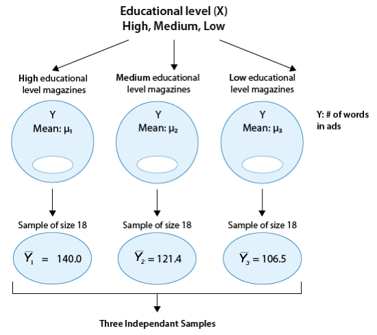
• Our question of interest is whether the number of words in ads (Y) is related to the educational level of the magazine (X). To answer this question, we need to compare \( \mu_1, \mu_2, \mu_3 \), the mean number of words in ads of the three magazine groups. Note in the figure that the sample means are provided. It seems that what the data suggest makes sense; the magazines in group 1 have the largest number of words per ad (on average) followed by group 2, and then group 3.




• The question is whether these differences between the sample means are significant. In other words, are the differences among the observed sample means due to true differences among the μ's or merely due to sampling variability? To answer this question, we need to carry out the ANOVA F-test.




• Step 1: Stating the hypotheses. We are testing:




• 




• Conceptually, the null hypothesis claims that the number of words in ads is not related to the educational level of the magazine, and the alternative hypothesis claims that there is a relationship.




• Step 2: Checking conditions and summarizing the data.




1. (i) The ads were selected at random from each magazine group, so the three samples are independent.




2. In order to check the next two conditions, we'll need to look at the data (condition ii), and calculate the sample standard deviations of the three samples (condition iii). Here are the side-by-side boxplots of the data, followed by the standard deviations:




3. 




4. 




5. (ii) The graph does not display any alarming violations of the normality assumption. It seems like there is some skewness in groups 2 and 3, but not extremely so, and there are no outliers in the data.




6. (iii) We can assume that the equal standard deviation assumption is met since the rule of thumb is satisfied: the largest sample standard deviation of the three is 74 (group 1), the smallest one is 57.6 (group 3), and 74/57.6 < 2.




• Before we move on, let's look again at the graph. It is easy to see the trend of the sample means (indicated by red circles). However, there is so much variation within each of the groups that there is almost a complete overlap between the three boxplots, and the differences between the means are over-shadowed and seem like something that could have happened just by chance. Let's move on and see whether the ANOVA F-test will support this observation.




• Using statistical software to conduct the ANOVA F-test, we find that the F statistic is 1.18, which is not very large. We also find that the p-value is 0.317.




• Step 3. Finding the p-value.




1. The p-value is 0.317, which tells us that getting data like those observed is not very surprising assuming that there are no differences between the three magazine groups with respect to the mean number of words in ads (which is what Ho claims).




2. In other words, the large p-value tells us that it is quite reasonable that the differences between the observed sample means could have happened just by chance (i.e., due to sampling variability) and not because of true differences between the means.




• Step 4: Making conclusions in context.




1. The large p-value indicates that the results are not significant, and that we cannot reject Ho.




2. We therefore conclude that the study does not provide evidence that the mean number of words in ads is related to the educational level of the magazine. In other words, the study does not provide evidence that advertisers alter the reading level of their ads (as measured by the number of words) based on the educational level of the target audience of the magazine.

• The purpose of this activity is to give you guided practice in carrying out the ANOVA F-test.




• Background: Critical Flicker Frequency (CFF) and Eye Color




• There is various flickering light in our environment; for instance, light from computer screens and fluorescent bulbs. If the frequency of the flicker is below a certain threshold, the flicker can be detected by the eye. Different people have slightly different flicker "threshold" frequencies (known as the critical flicker frequency, or CFF). Knowing the critical threshold frequency below which flicker is detected can be important for product manufacturing as well as tests for ocular disease. Do people with different eye color have different threshold flicker sensitivity? A 1973 study This link opens in a new tab ("The Effect of Iris Color on Critical Flicker Frequency," Journal of General Psychology [1973], 91 - 95) obtained the following data from a random sample of 19 subjects.




• 




• Do these data suggest that people with different eye color have different threshold sensitivity to flickering light? In other words, do the data suggest that threshold sensitivity to flickering light is related to eye color?




• Comment: We recommend that before starting, you create for yourself a figure that summarizes this problem, similar to the figures that we presented for the examples that we used in this part.

Q. What is the explanatory variable (X) and how many values does it take? What are those values? What is the response variable (Y)?

• We want to check whether CFF is related to eye color, therefore, the explanatory variable is eye color, which takes three values: Brown, Green and Blue, and the response variable is CFF.

Q. What are the hypotheses that are being tested here? Be sure that you define clearly the parameters that you are using.

• The hypotheses that being tested here are: Ho: μ1 = μ2 = μ3 Ha: not all the μ's are equal Where: μ1 = mean CFF of people that have brown eyes. μ2 = mean CFF of people that have green eyes. μ3 = mean CFF of people that have blue eyes.

Q. Below are boxplots that show how the CFF values compare for the three different eye colors. 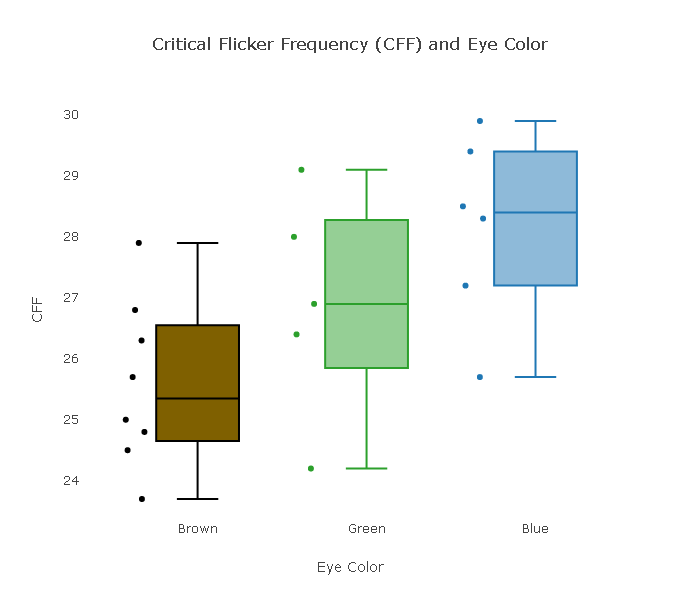The standard deviations for the various eye colors are: Brown: 1.365, Green: 1.843, and Blue: 1.527. Are the conditions that allow us to safely use the ANOVA F-test met?

• Let's check the conditions: (i) We are told that the sample was chosen at random, so the three eye-color samples are independent. (ii) The sample sizes are quite low, but the boxplots do not display any extreme violation of the normality assumption in the form of extreme skewness or outliers. (iii) We can assume that the equal population standard deviation condition is met, since the rule of thumb is satisfied (1.843 / 1.365 is less than 2).In summary, we can safely proceed with the ANOVA F-test.

Q. Based on the boxplots, summarize what the data suggest about how CFF is related to eye color. Do you think that the data provide enough evidence against the null hypothesis? (There is no right or wrong answer here, just your feelings from looking at the data.)

• The data suggest that the CFF of the people with brown eyes is the lowest (on average), followed by green-eyed people, and people with blue eyes have the highest CFF (on average). It seems like that there is a reasonable amount of evidence in the data against H0. The three boxplots do not overlap much, and it really doesn't seem very likely that the three populations from which these three samples were chosen all share the same mean.

Q. Here is the ANOVA F-test output. Interpret the p-value and draw your conclusion in context.

• The test statistic F is 4.8 (which is quite large), and the p-value is 0.023, indicating that it is unlikely (probability of 0.023) to get data like those observed assuming that CFF is not related to eye color (as the null hypothesis claims). Since the p-value is small (in particular, smaller than 0.05), we have enough evidence in the data to reject H0 and conclude that the mean CFFs in the three eye-color populations are not all the same. In other words, we can conclude that CFF is related to eye color.

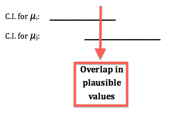
• However, the ANOVA F-test does not provide any insight into why H0 was rejected; it does not tell us in what way \( \mu_1, \mu_2, ... , \mu_k \) are not all equal. We would like to know which pairs of μs are not equal. As an exploratory (or visual) aid to get that insight, we may take a look at the confidence intervals for group population means \( \mu_1, \mu_2, ... , \mu_k \) that appears in the output. More specifically, we should look at the position of the confidence intervals and overlap / no overlap between them.




• * If the confidence interval for, say, \( \mu_i \) overlaps with the confidence interval for \( \mu_j \) , then \( \mu_i \) and \( \mu_j \) share some plausible values, which means that based on the data we have no evidence that these two μs are different.




• 




• * If the confidence interval for \( \mu_i \) does not overlap with the confidence interval for \( \mu_j \) , then \( \mu_i \) and \( \mu_j \) do not share plausible values, which means that the data suggest that these two μs are different.




• 




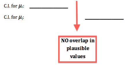
• Furthermore, if like in the figure above the confidence interval (set of plausible values) for \( \mu_i \) lies entirely below the confidence interval (set of plausible values) for \( \mu_j \), then the data suggest that \( \mu_i \) is smaller than \( \mu_j \).




• Example Consider our first example on the level of academic frustration.




1. 




2. Based on the small p-value, we rejected Ho and concluded that not all four frustration level means are equal, or in other words that frustration level is related to the student's major. To get more insight into that relationship, we can look at the confidence intervals above (marked in red). The top confidence interval is the set of plausible values for μ1, the mean frustration level of business students. The confidence interval below it is the set of plausible values for μ2, the mean frustration level of English students, etc.




3. What we see is that the business confidence interval is way below the other three (it doesn't overlap with any of them). The math confidence interval overlaps with both the English and the psychology confidence intervals; however, there is no overlap between the English and psychology confidence intervals.




4. This gives us the impression that the mean frustration level of business students is lower than the mean in the other three majors. Within the other three majors, we get the impression that the mean frustration of math students may not differ much from the mean of both English and psychology students, however the mean frustration of English students may be lower than the mean of psychology students.




5. Note that this is only an exploratory/visual way of getting an impression of why Ho was rejected, not a formal one. There is a formal way of doing it that is called "multiple comparisons," which is beyond the scope of this course. An extension to this course will include this topic in the future.




• Let's Summarize




1. The ANOVA F-test is used for comparing more than two population means when the samples (drawn from each of the populations we are comparing) are independent. We encounter this situation when we want to examine the relationship between a quantitative response variable and a categorical explanatory variable that has more than two values.




2. The hypotheses that are being tested in the ANOVA F-test are: \( H_0 : \mu_1 = \mu_2 = .. = \mu_k \) ; \( H_a : \text{not all μ are equal} \) The idea behind the ANOVA F-test is to check whether the variation among the sample means is due to true differences among the μ's or merely due to sampling variability by looking at: \( \frac{\text{variation among the sample means}}{\text{variation among the groups}} \)




3. Once we verify that we can safely proceed with the ANOVA F-test, we use software to carry it out.




4. If the ANOVA F-test has rejected the null hypothesis we can look at the confidence intervals for the population means that are in the output to get a visual insight into why Ho was rejected (i.e., which of the means differ).

Previous

Next