Inference for the Relationships between Two Categorical Variables (Chi-Square Test for Independence) : Overview
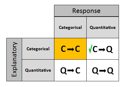
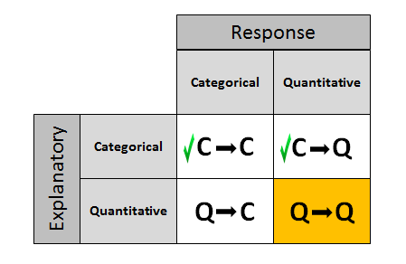
The last three procedures that we studied (two-sample t, paired t, and ANOVA) all involve the relationship between a categorical explanatory variable and a quantitative response variable, corresponding to Case C → Q in the role/type classification table below. Next, we will consider inferences about the relationships between two categorical variables, corresponding to case C → C.
In the Exploratory Data Analysis section of the course, we summarized the relationship between two categorical variables for a given data set (using a two-way table and conditional percents), without trying to generalize beyond the sample data.
Now we perform statistical inference for two categorical variables, using the sample data to draw conclusions about whether or not we have evidence that the variables are related in the larger population from which the sample was drawn. In other words, we would like to assess whether the relationship between X and Y that we observed in the data is due to a real relationship between X and Y in the population or if it is something that could have happened just by chance due to sampling variability.
The statistical test that will answer this question is called the chi-square test for independence. Chi is a Greek letter that looks like this: \( \chi \), so the test is sometimes referred to as: The \( \chi^2 \) test for independence.
The structure of this section will be very similar to that of the previous ones in this module. We will first present our leading example, and then introduce the chi-square test by going through its 4 steps, illustrating each one using the example. We will conclude by presenting another complete example. As usual, you'll have activities along the way to check your understanding, and to learn how to use software to carry out the test.
Example
In the early 1970s, a young man challenged an Oklahoma state law that prohibited the sale of 3.2% beer to males under age 21 but allowed its sale to females in the same age group. The case (Craig v. Boren, 429 U.S. 190, 1976) was ultimately heard by the U.S. Supreme Court.
The main justification provided by Oklahoma for the law was traffic safety. One of the 3 main pieces of data presented to the court was the result of a "random roadside survey" that recorded information on gender, and whether or not the driver had been drinking alcohol in the previous two hours. There were a total of 619 drivers under 20 years of age included in the survey.
Here is what the collected data looked like:
The following two-way table summarizes the observed counts in the roadside survey:
Our task is to assess whether these results provide evidence of a significant ("real") relationship between gender and drunk driving.
The following figure summarizes this example:
Note that as the figure stresses, since we are looking to see whether drunk driving is related to gender, our explanatory variable (X) is gender, and the response variable (Y) is drunk driving. Both variables are two-valued categorical variables, and therefore our two-way table of observed counts is 2-by-2. It should be mentioned that the chi-square procedure that we are going to introduce here is not limited to 2-by-2 situations, but can be applied to any r-by-c situation where r is the number of rows (corresponding to the number of values of one of the variables) and c is the number of columns (corresponding to the number of values of the other variable).
Before we introduce the chi-square test, let's conduct an exploratory data analysis (that is, look at the data to get an initial feel for it). By doing that, we will also get a better conceptual understanding of the role of the test.
Exploratory Analysis
Recall that the key to reporting appropriate summaries for a two-way table is deciding which of the two categorical variables plays the role of explanatory variable, and then calculating the conditional percentages — the percentages of the response variable for each value of the explanatory variable — separately. In this case, since the explanatory variable is gender, we would calculate the percentages of drivers who did (and did not) drink alcohol for males and females separately.
Here is the table of conditional percentages:
For the 619 sampled drivers, a larger percentage of males were found to be drunk than females (16.0% vs. 11.6%). Our data, in other words, provide some evidence that drunk driving is related to gender; however, this in itself is not enough to conclude that such a relationship exists in the larger population of drivers under 20. We need to further investigate the data and decide between the following two points of view:
The evidence provided by the roadside survey (16% vs 11.6%) is strong enough to conclude (beyond a reasonable doubt) that it must be due to a relationship between drunk driving and gender in the population of drivers under 20.
The evidence provided by the roadside survey (16% vs. 11.6%) is not strong enough to make that conclusion, and could have happened just by chance, due to sampling variability, and not necessarily because a relationship exists in the population.
Actually, these two opposing points of view constitute the null and alternative hypotheses of the chi-square test for independence, so now that we understand our example and what we still need to find out, let's introduce the four-step process of this test.
Scenario: Alcoholism Risk in 9/11 Responders
The purpose of this activity is to introduce you to the example that you are going to work through in this section, and for you to get a feeling for the data by conducting exploratory analysis.
Background: Alcoholism Risk in 9/11 Responders
Among firefighters and other "first responders" to the World Trade Center on September 11, 2001, there have been reports of increased alcohol-related difficulties (e.g., DUI). A survey of 9/11 first responders (On the Front Line: The Work of First Responders in a Post-9/11 World) conducted by Cornell researcher Samuel Bacharach was released in 2004. To see the report, click here This link opens in a new tab. Based on the research, we can construct the following two-way table of observed counts:
Using the data from this research, we would like to investigate whether alcohol risk among New York firefighters is significantly related to participation in the 9/11 rescue.
Q. There are two categorical variables in this problem:* Alcohol risk (none, moderate to severe)* Participation in the 9/11 rescue (yes, no)Which is the explanatory variable and which is the response?
Since we want to investigate whether participation in the 9/11 rescue had an effect on alcohol risk, the explanatory variable is "participation in the 9/11 rescue" and the response variable is "alcohol risk."
Q. Conduct exploratory analysis of the data by calculating the conditional percentages. Summarize your findings. Recall that we calculate the percentages of the response variable for each category of the explanatory variable separately.
According to our data, a larger percentage of the firefighters who participated in the 9/11 rescue are at risk for alcohol problems compared to the percentage among firefighters who did not participate in the 9/11 rescue (28% vs. 20%).
The question now is whether this difference in the percentages is significant or not.
In other words, the next step would be to carry out a significance test that will assess whether observing data like ours (where there is a difference of 8% between the firefighters who participated in the 9/11 rescue and those who didn't) is likely to happen just by chance or the fact the we observed these data provides enough evidence that the risk of alcohol-related problems among New York firefighters and first responders is indeed related to participation in the 9/11 rescue.
Case C → C: The Idea of the Chi-Square Test
The chi-square test for independence examines our observed data and tells us whether we have enough evidence to conclude beyond a reasonable doubt that two categorical variables are related. Much like the previous part on the ANOVA F-test, we are going to introduce the hypotheses (step 1), and then discuss the idea behind the test, which will naturally lead to the test statistic (step 2). Let's start.
Step 1: Stating the hypotheses Unlike all the previous tests that we presented, the null and alternative hypotheses in the chi-square test are stated in words rather than in terms of population parameters. They are:
Ho: There is no relationship between the two categorical variables. (They are independent.)
Ha: There is a relationship between the two categorical variables. (They are not independent.)
Example : In our example, the null and alternative hypotheses would then state:
Ho: There is no relationship between gender and drunk driving.
Ha: There is a relationship between gender and drunk driving.
Or equivalently,
Ho: Drunk driving and gender are independent
Ha: Drunk driving and gender are not independent
and hence the name "chi-square test for independence."
Comment
Algebraically, independence between gender and driving drunk is equivalent to having equal proportions who drank (or did not drink) for males vs. females. In fact, the null and alternative hypotheses could have been re-formulated as
Ho: proportion of male drunk drivers = proportion of female drunk drivers
Ha: proportion of male drunk drivers ≠ proportion of female drunk drivers
However, expressing the hypotheses in terms of proportions works well and is quite intuitive for two-by-two tables, but the formulation becomes very cumbersome when at least one of the variables has several possible values, not just two. We are therefore going to always stick with the "wordy" form of the hypotheses presented in step 1 above.
The Idea of the Chi-Square Test
The idea behind the chi-square test, much like previous tests that we've introduced, is to measure how far the data are from what is claimed in the null hypothesis. The further the data are from the null hypothesis, the more evidence the data presents against it. We'll use our data to develop this idea. Our data are represented by the observed counts:
How will we represent the null hypothesis?
In the previous tests we introduced, the null hypothesis was represented by the null value. Here there is not really a null value, but rather a claim that the two categorical variables (drunk driving and gender, in this case) are independent.
To represent the null hypothesis, we will calculate another set of counts — the counts that we would expect to see (instead of the observed ones) if drunk driving and gender were really independent (i.e., if Ho were true). For example, we actually observed 77 males who drove drunk; if drunk driving and gender were indeed independent (if Ho were true), how many male drunk drivers would we expect to see instead of 77? Similarly, we can ask the same kind of question about (and calculate) the other three cells in our table.
In other words, we will have two sets of counts:
the observed counts (the data)
the expected counts (if Ho were true)
We will measure how far the observed counts are from the expected ones. Ultimately, we will base our decision on the size of the discrepancy between what we observed and what we would expect to observe if Ho were true.
How are the expected counts calculated? Once again, we are in need of probability results. Recall from the probability section that if events A and B are independent, then P(A and B) = P(A) * P(B). We use this rule for calculating expected counts, one cell at a time. Here again are the observed counts:
Applying the rule to the first (top left) cell, if driving drunk and gender were independent then: P(drunk and male) = P(drunk) * P(male)
By dividing the counts in our table, we see that:
P(Drunk) = 93 / 619 and
P(Male) = 481 / 619,
P(Drunk and Male) = (93 / 619) (481 / 619)
Therefore, since there are total of 619 drivers, if drunk driving and gender were independent, the count of drunk male drivers that I would expect to see is: \( 619 * \text{P(Drunk and male)} = 619 * \frac{93}{619} * \frac{481}{619} = \frac{93*481}{619} \)
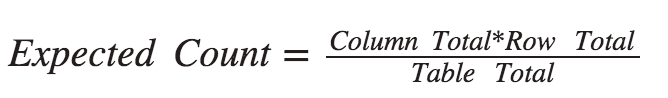
Notice that this expression is the product of the column and row totals for that particular cell, divided by the overall table total.
Similarly, if the variables are independent,
P(Drunk and Female) = P(Drunk) * P(Female) = (93 / 619) (138 / 619)
and the expected count of females driving drunk would be \( \frac{93}{619} * \frac{138}{619} = \frac{93*138}{619} \)
Again, the expected count equals the product of the corresponding column and row totals, divided by the overall table total:
This will always be the case, and will help streamline our calculations: \( \text{Expected count} = \frac{\text{Column total * Row total}}{\text{Table total}} \)
- Explanation :
Indeed 526 is the column total for this cell, and 481 is the row total.
- Explanation :
Indeed, 526 is the column total for this cell, and 138 is the row total.
Complete table of expected counts, followed by the table of observed counts
Scenario: Gender and Ear Piercing
A study was done on the relationship between gender and piercing among high-school students. A sample of 1,000 students was chosen, then classified according to gender and according to whether or not they had any of their ears pierced. The results of the study are summarized in the following 2-by-2 table:
We see that there are differences between the observed and expected counts in the respective cells. We now have to come up with a measure that will quantify these differences. This is the chi-square test statistic.
- Explanation :
Indeed, the expected count of non-pierced females is (640 * 352) / 1,000 = 225.28
- Explanation :
The expected count is the number of non-pierced females if the null hypothesis were true and the null hypothesis were true.
Case C → C: Conditions and Chi-Square Test
Step 2: Checking the Conditions and Calculating the Test Statistic Given our discussion on the previous page, it would be natural to present the test statistic, and then come back to the conditions that allow us to safely use the chi-square test, although in practice this is done the other way around.
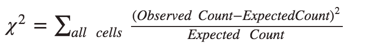
The single number that summarizes the overall difference between observed and expected counts is the chi-square statistic \( \chi^2 \) , which tells us in a standardized way how far what we observed (data) is from what would be expected if Ho were true.
Here it is: \( \chi^2 = \sum_{all cells} \frac{\text{Observed count - Expected count}^2}{\text{Expeced count}}\)
Comment
As we expected, \( \chi^2 \) is based on each of the differences: observed count - expected count (one such difference for each cell), but why is it squared? Why do we divide each square difference by the expected count? The reason we do that is so that the null distribution of \( \chi^2 \) will have a known null distribution (under which p-values can be easily calculated). The details are really beyond the scope of this course, but we will just say that the null distribution of \( \chi^2 \) is called chi-square (which is not very surprising given that the test is called the chi-square test), and like the t-distributions there are many chi-square distributions distinguished by the number of degrees of freedom associated with them.
Conditions under Which the Chi-Square Test Can Safely Be Used - The sample should be random.
In general, the larger the sample, the more accurate and reliable the test results are. There are different versions of what the conditions are that will ensure reliable use of the test, all of which involve the expected counts. One version of the conditions says that all expected counts need to be greater than 1, and at least 80% of expected counts need to be greater than 5. A more conservative version requires that all expected counts are larger than 5.
Example :Here, again, are the observed and expected counts.
Checking the conditions:
The roadside survey is known to have been random.
All the expected counts are above 5.
We can therefore safely proceed with the chi-square test, and the chi-square test statistic is: \( \frac{(77-72.3)^2}{72.3} + \frac{(404-408.7)^2}{408.7} + \frac{(16-20.7)^2}{20.7} + \frac{(122-117.3)^2}{117.3} = 0.306 + 0.054 + 1.067 + 0.188 = 1.62 \)
Scenario: Ear Piercing and Gender
A study was done on the relationship between gender and piercing among high-school students. A sample of 1,000 students was chosen, and then classified according to both gender and whether or not they had either of their ears pierced. The following (edited) output is available:
- Explanation :
Indeed, the contribution of the first cell is (observed count - expected count)2 / expected count = (576 - 414.72)2 / 414.72 = 62.72.
- Explanation :
The contribution of the fourth cell (no-pierced males) to the chi-square statistic is: (Observed - Expected)2/Expected = (288-126.72)2 / 126.72 = 205.27
- Explanation :
Indeed, to find the test statistic, we need to add the contributions of each of the 4 cells, which in this case is: 62.72 + 115.462 + 111.502 + 205.265 = 494.949
Comment
Once the chi-square statistic has been calculated, we can get a feel for its size: is there a relatively large difference between what we observed and what the null hypothesis claims, or a relatively small one?
It turns out that for a 2-by-2 case like ours, we are inclined to call the chi-square statistic "large" if it is larger than 3.84.
Therefore, our test statistic is not large, indicating that the data are not different enough from the null hypothesis for us to reject it (we will also see that in the p-value not being small).
For other cases (other than 2-by-2) there are different cut-offs for what is considered large, which are determined by the null distribution in that case.
We are therefore going to rely only on the p-value to draw our conclusions.
Even though we cannot really use the chi-square statistic, it was important to learn about it, since it encompasses the idea behind the test
Scenario: Alcohol Problems Among 9/11 First Responders
The purpose of this activity is to continue to explore whether the risk of alcohol problems among New York firefighters and first responders is related to participation in the 911 rescue. In particular, in this activity, we will state the hypotheses that are being tested, learn how to carry out the chi-square test for independence, and check whether the conditions under which this test can be safely used are met.
Observed Data No risk for alchohol problems Moderate to Servere risk for alcohol problems Total Participated in 911 rescue 793 309 1102 Did Not Participate in 911 rescue 441 110 551 Total 1234 419 1653
- Explanation :
Either format can be used to describe the null and alternative hypotheses for the chi-square test for independence. One way is to state that the null hypothesis can be no relationship between the two variables and the alternative hypothesis is that there is a significant relationship between the two variables. A second way is to state that the null hypothesis is that the two variables are independent and the alternative hypothesis is the two variables are not independent.
- Explanation :
According to the report, the sample was stratified using randomness. • As the output shows, all the expected counts are large.
Case C → C: Finding the p-value
Step 3: Finding the p-value
The p-value for the chi-square test for independence is the probability of getting counts like those observed, assuming that the two variables are not related (which is what is claimed by the null hypothesis). The smaller the p-value, the more surprising it would be to get counts like we did, if the null hypothesis were true.
Technically, the p-value is the probability of observing \( \chi^2 \) at least as large as the one observed. Using statistical software, we find that the p-value for this test is 0.201.
Step 4: Stating the conclusion in context
As usual, we use the magnitude of the p-value to draw our conclusions. A small p-value indicates that the evidence provided by the data is strong enough to reject Ho and conclude (beyond a reasonable doubt) that the two variables are related. In particular, if a significance level of 0.05 is used, we will reject Ho if the p-value is less than 0.05.
Example
A p-value of 0.201 is not small at all. There is no compelling statistical evidence to reject Ho, and so we will continue to assume it may be true. Gender and drunk driving may be independent, and so the data suggest that a law that forbids sale of 3.2% beer to males and permits it to females is unwarranted. In fact, the Supreme Court, by a 7-2 majority, struck down the Oklahoma law as discriminatory and unjustified. In the majority opinion Justice Brennan wrote :
"Clearly, the protection of public health and safety represents an important function of state and local governments. However, appellees' statistics in our view cannot support the conclusion that the gender-based distinction closely serves to achieve that objective and therefore the distinction cannot under [prior case law] withstand equal protection challenge."
Scenario: Alcohol Problems Among 9/11 First Responders
The purpose of this activity is to draw our conclusion regarding the relationship between participation in the 9/11 rescue and risk of alcohol problems among New York firefighters and first responders.
A chi-square test regarding the relationship between participation in the 9/11 rescue and risk of alcohol problems among New York firefighters and first responders produced the following results:
- Explanation :
In order to reject the null hypothesis of no relationship between two categorical variables, the p-value must be less than 0.05. The calculated p-value of 0.0004 is less than 0.05; therefore, the null hypothesis should be rejected and the conclusion drawn that there is a relationship between alcohol problems in New York firefighters and participation in the 9/11 rescue.
Case C → C: Finding the p-value
Comment
This is a good opportunity to illustrate an important idea that was discussed earlier in this unit: The larger the sample the results are based on, the more evidence they carry. Let's take the previous example and simply multiply each of the counts by 3:
and see what would have happened if these were the original data. Obviously, the conditional counts would remain the same:
In other words, the sample provides the "same" results, but this time they are based on a much larger sample (1857 instead of 619). This is reflected by the chi-square test. In this case, software gives us a chi-square statistic of 4.910 and a p-value of 0.027.
As before, Ho states that gender and drunk driving are not related; Ha states that they are related. Since the observed counts are triple what they were before, the expected counts are also tripled. When done with software the original chi-square statistic was 1.637 since software doesn't round as much. The chi-square statistic when we tripled the data is 3 times 1.637, or 4.91 (which now is in the "large" range). Therefore, the p-value is smaller and is now .027.
Now, we do reject Ho, and we conclude that gender and drunk driving are related. In this case, the "largest contribution to chi-square" is large enough to provide evidence of a relationship. This is due to the fact that so few females drove drunk (48) compared to the number that would be expected (62.2, which is 414 * 279 / 1857) if the variables gender and drunk driving were not related. This contribution is \( \frac{(48-62.2)^2}{62.2} = 3.242\).
- Explanation :
In order to reject the null hypothesis of no relationship between two categorical variables, the p-value must be less than 0.05. The calculated p-value of 0.0004 is less than 0.05; therefore, the null hypothesis should be rejected and the conclusion drawn that there is a relationship between alcohol problems in New York firefighters and participation in the 9/11 rescue.
Case C → C: Summary (Steroid Use in Sports)
Major-league baseball star Barry Bonds admitted to using a steroid cream during the 2003 season. Is steroid use different in baseball than in other sports? According to the 2001 National Collegiate Athletic Association (NCAA) survey , which is self-reported and asked of a stratified random selection of teams from each of the three NCAA divisions, reported steroid use among the top 5 college sports was as follows:
Do the data provide evidence of a significant relationship between steroid use and the type of sport? In other words, are there significant differences in steroid use among the different sports?
Before we carry out the chi-square test for independence, let's get a sense of the data by calculating the conditional percents:
It seems as if there are differences in steroid use among the different sports. Even though the differences do not seem to be overwhelming, since the sample size is so large, these differences might be significant. Let's carry out the test and see.
Step 1: Stating the hypotheses
The hypotheses are:
H0: steroid use is not related to the type of sport (or: type of sport and steroid use are independent)
Ha: Steroid use is related to the type of sport (or: type of sport and steroid use are not independent).
Step 2: Checking conditions and finding the test statistic
Here is the statistical software output of the chi-square test for this example:
Conditions:
We are told that the sample was random.
All the expected counts are above 5.
Test statistic: The test statistic is 14.626. Note that the "largest contributors" to the test statistic are 5.729 and 3.990. The first cell corresponds to football players who used steroids, with an observed count larger than we would expect to see under independence. The second cell corresponds to tennis players who used steroids, and has an observed count lower than we would expect under independence.
Step 3: Finding the p-value - According to the output p-value it would be extremely unlikely (probability of 0.006) to get counts like those observed if the null hypothesis were true. In other words, it would be very surprising to get data like those observed if steroid use were not related to sport type.
Step 4: Conclusion - The small p-value indicates that the data provide strong evidence against the null hypothesis, so we reject it and conclude that the steroid use is related to the type of sport.
Let's Summarize
The chi-square test for independence is used to test whether the relationship between two categorical variables is significant. In other words, the chi-square procedure assesses whether the data provide enough evidence that a true relationship between the two variables exists in the population.
The hypotheses that are being tested in the chi-square test for independence are:
H0: There is no relationship between ... and ....
Ha: There is a relationship between ... and ....
or equivalently,
H0: The variables ... and ... are independent.
Ha: The variables ... and ... are not independent.
The idea behind the test is measuring how far the observed data are from the null hypothesis by comparing the observed counts to the expected counts—the counts that we would expect to see (instead of the observed ones) had the null hypothesis been true. The expected count of each cell is calculated as follows:
The measure of the difference between the observed and expected counts is the chi-square test statistic, whose null distribution is called the chi-square distribution. The chi-square test statistic is calculated as follows:
Once we verify that the conditions that allow us to safely use the chi-square test are met, we use software to carry it out and use the p-value to guide our conclusions
Inference for the Linear Relationships between Two Quantitative Variables - Case Q → Q: Overview
In inference for relationships, so far we have learned inference procedures for both cases C → Q and C → C from the role/type classification table below. The last case to be considered in this course is case Q → Q, where both the explanatory and response variables are quantitative. (Case Q → C requires statistical methods that go beyond the scope of this course, but might be part of extension modules in the future).
In the Exploratory Data Analysis section, we examined the relationship between sample values for two quantitative variables by looking at a scatterplot and focused on the linear relationship by supplementing the scatterplot with the correlation coefficient r.
There was no attempt made to claim that whatever relationship was observed in the sample necessarily held for the larger population from which the sample originated. Now that we have a better understanding of the process of statistical inference, we will present the method for inferring something about the relationship between two quantitative variables in an entire population, based on the relationship seen in the sample. In particular, the method will focus on linear relationships and will answer the following question: Is the observed linear relationship due to a true linear relationship between two variables in the population, or could it be that we obtained this kind of pattern in the data just by chance?
If we conclude that we can generalize the observed linear relationship to the entire population, we will then use the data to estimate the line that governs the linear relationship between the two variables in the population, and use it to make predictions. The following figure summarizes this process:
Note that the figure summarizes the whole process. Let's review it again.
We start by asking whether the two quantitative variables are related (in any way).
We collect data, and when we summarize them with a scatterplot and the correlation r, we observe a linear relationship.
Then we get to the inference part of the process, which we are going to learn here:
We will carry out a test that will tell us whether the observed linear relationship is significant (i.e., can be generalized to the entire population).
If the observed linear relationship is not significant—too bad.
If the observed linear relationship is significant, we can use the data to estimate the line that governs the linear relationship between X and Y in the population, and can use it to make predictions (see comment 1 below).
Comments
We estimate the line that governs the linear relationship between X and Y in the population by the line that best fits the linear pattern in our observed data. Recall that in the Exploratory Data Analysis unit we've actually already learned how to find the least squares regression line—the line that best fits the observed data. You can now see that finding the least squares regression line actually belongs to the inference unit, and while it is true that it is the line that best fits (in some sense) the observed data, it is really an estimate of the true linear relationship that exists in the population. The good thing is that we already learned how to obtain this line, so we'll only need to review it.
This section on regression will be very qualitative in nature and will rely mostly on conceptual ideas and on output. An extension module to this course, which will go deeper into the inferential processes of regression, will exist in the near future.
This section will be organized around a leading example. At some stages along the way, you'll be directed to an activity, where you'll get to have hands-on practice with a different example.
Case Q → Q: Hypotheses to Conclusion
Let's introduce our leading example, which was actually our leading example in the Exploratory Data Analysis section as well.
Example In a study of the legibility and visibility of highway signs, a Pennsylvania research firm determined the maximum distance at which each of 30 drivers could read a newly designed sign. The 30 participants in the study ranged in age from 18 to 82 years old. The government agency that funded the research hoped to improve highway safety for older drivers and wanted to examine the relationship between age and sign legibility distance. (Data adopted with permission from Utts and Heckard, Mind on Statistics).
Let's go through the entire process (outlined on the previous page) for this example.
Starting point: The researchers wanted to examine the relationship between age and sign legibility distance in the population of drivers. The researchers collected data from a random sample of 30 drivers:
Exploratory Analysis:
The researchers display the data on a scatterplot:
and observe a negative linear relationship in the data. In order to quantify the strength of that linear relationship, the researchers supplement the scatterplot with a numerical measure—the correlation coefficient (r), which turns out to be r = -0.801, confirming the researchers' visual assessment of a negative, fairly strong linear relationship between age and legibility distance.
Scenario: Infant Vocalization and IQ
The purpose of this activity is to introduce the example that you will work on in the activities of this section and to have you get a first feel for the data via exploratory data analysis.
Background: A method for predicting IQ as soon as possible after birth could be important for early intervention in cases such as brain abnormalities or learning disabilities. It has been thought that greater infant vocalization (for instance, more crying) is associated with higher IQ. In 1964, a study was undertaken to see if IQ at 3 years of age is associated with amount of crying at newborn age (Karelitz, et al., "Relation of Crying Activity in Early Infancy to Speech and Intellectual Development at Age Three Years," Child Development, 1964 (35), p. 769–777. Click here This link opens in a new tab to read the research paper that describes this study and its results).
In the study, 38 newborns were made to cry after being tapped on the foot, and the number of distinct cry vocalizations within 20 seconds was counted. The subjects were followed up at 3 years of age and their IQs were measured.
Here is what the data look like:
Cry Count IQ 1 10 87 2 20 90 3 17 94 4 12 94 5 12 97 6 15 100 7 19 103 8 12 103 9 14 103 10 23 103 11 15 104 12 14 106 13 13 106 14 27 108 15 17 109 16 12 109 17 18 109 18 15 112 19 15 112 20 23 113 21 16 114 22 21 114 23 16 118 24 12 119 25 9 119 26 13 120 27 19 120 28 18 124 29 19 132 30 16 133 31 22 135 32 31 135 33 16 136 34 17 141 35 26 155 36 21 157 37 27 159 38 13 162 As you can see, our data consist of two variables: cry count and IQ.
Q. Which is the explanatory variable and which is the response?
Since we want to examine how the vocalization of newborns can explain IQ at age three, the explanatory variable is cry count and the response variable is IQ.
Q. To get a feel for the data, we conduct exploratory analysis by creating a scatterplot of the data, and supplement it with the correlation coefficient r.
Here is the scatterplot:
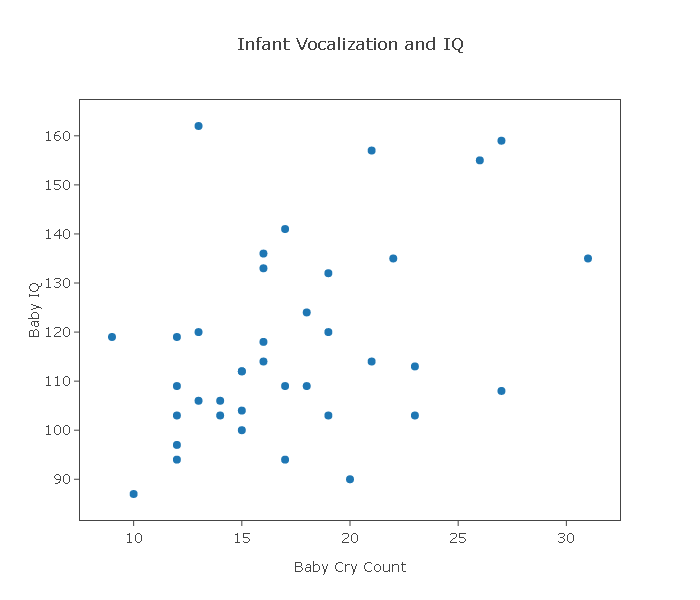 Using statistics software we find the correlation value to be 0.4018185. Based on the analysis above, comment on the direction, form, and strength of the relationship.
From the scatterplot we see that there is a general trend of a positive relationship between cry count and IQ, and that this relationship seems to be linear but quite weak. In order to quantify the strength of the linear relationship, we supplement the scatterplot with r, which turns out to be roughly 0.4. The value of r tells us that the linear relationship between cry count and IQ is weak to moderate.
Inference
The researchers would now like to see whether the observed linear relationship between age and legibility distance can be generalized to the entire population of drivers. In other words, the researchers want to check whether the observed linearity is due to true linearity in the population, or a pattern that could have happened just by chance.
The test that the researchers are going to carry out is a t-test (most commonly known as the "t-test for the slope" for reasons that we are not going to get into) which is testing the following two hypotheses (step 1):
Ho: There is no linear relationship between age and distance.
Ha: There is a linear relationship between age and distance.
and in general,
Ho: There is no linear relationship between X and Y.
Ha: There is a linear relationship between X and Y.
- Explanation :
These hypotheses correctly describe the type of relationship, i.e. linear. Also, the null hypothesis correctly indicates no relationship and the alternative hypothesis correctly indicates a relationship.
- Explanation :
These hypotheses correctly describe the type of relationship, i.e. linear. Also, the null hypothesis correctly indicates no relationship and the alternative hypothesis correctly indicates a relationship.
Comments
. As we mentioned earlier, we are going to keep this discussion on the qualitative side and in particular we will not go very deeply into step 2 of the hypothesis test. As for the test-statistic in this case, we'll just say that the test is a t-test, which, as we know, means that the null distribution of its test statistic (under which the p-values are calculated) is some t distribution.
We are also going to focus on only some of the conditions that allow us to safely use this t-test. They are:
the observed data indeed look linear (otherwise it would not make sense to try and generalize them)
the observations are independent
there are no extreme outliers in the data
the sample size is fairly large
Note that in our example all these conditions are met; the data definitely look linear, the observations (drivers) are independent of each other (since they were randomly chosen), there are no extreme observations in the data, and a sample size of n = 30 is fairly large.
For step 3, the researchers use statistical software to find a test statistic value of -7.09, and a p-value that is so small that it is essentially 0. This means that it would be extremely unlikely (actually, quite impossible) to get data like those observed if age and legibility distance were not linearly related. In other words, it would be extremely unlikely to get data like those observed just by chance.
The researchers conclude (step 4) that since the p-value is so small, the data provide extremely strong evidence to reject Ho and conclude that age and legibility distance are linearly related.
- Explanation :
With a p-value < 0.05, we would reject the null hypothesis of no linear relationship.
- Explanation :
With a p-value < 0.05, we would reject the null hypothesis of no linear relationship.
- Explanation :
When the p-value > 0.05 we cannot reject the null hypothesis (we do not have sufficient evidence to reject the hypothesis of no significant linear relationship).
- Explanation :
When the p-value > 0.05 we cannot reject the null hypothesis (we do not have sufficient evidence to reject the hypothesis of no significant linear relationship).
Scenario: Infant Vocalization and IQ
The purpose of this activity is to give you guided practice in testing whether the data provide evidence of a significant linear relationship, and in verifying that the basic conditions under which the results of such a test are reliable are met.
Recall the example from the previous activity:
A method for predicting IQ as soon as possible after birth could be important for early intervention in cases such as brain abnormalities or learning disabilities. It has been thought that greater infant vocalization (for instance, more crying) is associated with higher IQ. In 1964, a study was undertaken to see if IQ at 3 years of age is associated with amount of crying at newborn age. In the study, 38 newborns were made to cry after being tapped on the foot and the number of distinct cry vocalizations within 20 seconds was counted. The subjects were followed up at 3 years of age and their IQs were measured.
We would now like to test whether the observed (weak-to-moderate) linear relationship between cry count and IQ is significant (in other words, we would like to carry out the "t-test for the slope" for this example)
- Explanation :
This is the appropriate *null* hypothesis, Ho. The appropriate alternative hypothesis is Ha: There is a significant linear relationship between cry count and IQ
- Explanation :
Independence is one of the conditions that must be met. According to the paper, the 38 infants were a sample of infants born at the Long Island Jewish Hospital at the time of the study. Given this information, we can assume that the observations are independent (even though it doesn't explicitly say that the sample was random). The only obvious way that the independence assumption would be violated is if twins (or triplets ...) were included in the study, which we can assume was not the case. Also, the relationship between the explanatory and response variable should be linear. In this example, the relationship seems linear (even though it is moderately weak). Additionally, there should be no extreme outliers. Lastly, the sample size should be reasonably large. In this example, sample size meets this condition (n = 38).
- Explanation :
The p-value of the test is 0.012. The small p-value (in particular, smaller than .05) tells us that it would be quite unlikely (1.2% chance) to get data like those observed just by chance. The data, therefore provide enough evidence for us to conclude that there is a significant linear relationship among infants between vocalization right after birth (as measured by cry count) and IQ at age 3.
Note:
It is important to distinguish between the information provided by r and by the p-value. The correlation coefficient r informs us about the strength of the linear relationship in the data: close to +1 or -1 for a strong linear relationship, close to 0 for a weak linear relationship. In contrast, the regression p-value informs us about the strength of evidence that there is a linear relationship in the population from which the data were obtained.
In our example, since the p-value is 0.000 and r = -0.801, we would say that we have extremely strong evidence of a fairly strong relationship between age and distance in the population of drivers.
- Explanation :
Indeed, r = 0.4 indicates that there is a moderately weak linear relationship between cry count and IQ in our data. In addition, the small p-value (0.012) tells us that these data provide fairly strong evidence that this linear relationship can be generalized to infants in the population.
Case Q → Q: Summary
So far, the researchers have observed linearity in the data, and based on a test concluded that this linear relationship between age and legibility distance can be generalized to the entire population of drivers.
Since that is the case, the researchers would now like to estimate the equation of the straight line that governs the linear relationship between age and legibility distance among drivers. As we commented earlier, this is done by finding the line that best fits the pattern of our observed data. Recall that this line is called the least squares regression line, which is the line that minimizes the sum of the squared vertical deviations:
In the Exploratory Data Analysis section, we presented the actual formulas for the slope and intercept of the line. We are not going to repeat those here; we will obtain those values from the output:
and ask the software to plot it for us on the scatterplot so we can see how well it fits the data.
Based on the observed data, the researchers conclude that the linear relationship between age and legibility distance among drivers can be summarized with the line:
DISTANCE = 576.7 - 3.007 * AGE
In particular, the slope of the line is roughly -3, which means that for every year that a driver gets older (1 unit increase in X), the maximum legibility distance is reduced, on average, by 3 feet (Y changes by the value of the slope).
The researchers can also use this line to make predictions, remembering to beware of extrapolations (predictions for X values that are outside of the range of the original data). For example, using the equation of the line, we predict that the maximum legibility distance of a 60-year-old driver is: distance = 576.7 - 3.007(60) = 396.28. The following figure illustrates this prediction.
Scenario: Infant Vocalization and IQ
The purpose of this activity is to complete our discussion about our example that examines the relationship between vocalization soon after birth and IQ at age three.
So far we explored the data using a scatterplot supplemented with the correlation r and discovered that the data display a moderately weak positive linear relationship.
In addition, when we carried out the t-test for assessing the significance of this linear relationship and we concluded (based on the small p-value of 0.012) that the data provide fairly strong evidence of a moderately weak linear relationship between cry count soon after birth and IQ and age 3.
We would now liketo consider using the least squares regression line for predicting IQ at age 3 based on cry count soon after birth. Below is the least squared regression line plotted on the scatterplot.
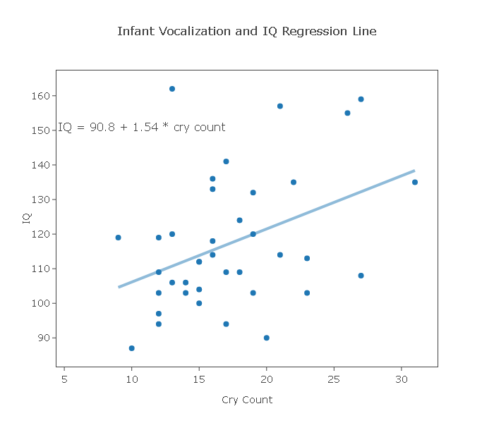
- Explanation :
The least squares regression line does not fit the data very well due to the moderately weak linearity in the data. Visually, we see that the data points do not lay close to the line, resulting in a relatively poor fit of the line to the data.
Simple linear regression results
Dependent Variable: IQ
Independent Variable: cry count
IQ = 90.75499 + 1.5363518 * cry count
Parameter Estimate Std. Err. Alternative DF T-Stat P-Value Intercept 90.75499 10.47342 ≠ 0 36 8.665267 < 0.0001 Slope 1.5363518 0.5835417 ≠ 0 36 2.6328056 0.0124
- Explanation :
The predicted IQ is obtained by plugging in a cry count of 19 into the regression line. We therefore obtain: Predicted IQ = 90.8 + 1.54 * 19 = 120.1.
Summarize
In the t-test for the significance of the linear relationship between two quantitative variables X and Y, we are testing
Ho: No linear relationship exists between X and Y.
Ha: A linear relationship exists between X and Y.
The test assesses the strength of evidence provided by the data (as seen in the scatterplot and measured by the correlation r) and reports a p-value. The p-value is the probability of getting data such as that observed assuming that, in reality, no linear relationship exists between X and Y in the population.
Based on the p-value, we draw our conclusions. A small p-value will indicate that we reject Ho and conclude that the data provide enough evidence of a real linear relationship between X and Y in the population.