What are matrices and what are vectors
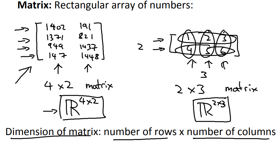
A matrix is a rectangular array of numbers written between square brackets. A matrix is just another way for saying, is a 2D or a two dimensional array. The dimension of the matrix is going to be written as the number of row times the number of columns in the matrix.
Matrices and Vectors
Matrices are 2-dimensional arrays:
\( \begin{bmatrix} a & b & c \newline d & e & f \newline g & h & i \newline j & k & l\end{bmatrix} \)
The above matrix has four rows and three columns, so it is a 4 x 3 matrix.
A vector is a matrix with one column and many rows:
\( \begin{bmatrix} w \newline x \newline y \newline z \end{bmatrix} \)
So vectors are a subset of matrices. The above vector is a 4 x 1 matrix.
Notation and terms:
\( A_{ij} \) - refers to the element in the ith row and jth column of matrix A.
A vector with 'n' rows is referred to as an 'n'-dimensional vector.
\( v_iv \)- refers to the element in the ith row of the vector.
In general, all our vectors and matrices will be 1-indexed. Note that for some programming languages, the arrays are 0-indexed.
Matrices are usually denoted by uppercase names while vectors are lowercase.
"Scalar" means that an object is a single value, not a vector or matrix.
\( \mathbb{R} \) refers to the set of scalar real numbers.
\( \mathbb{R^n} \) refers to the set of n-dimensional vectors of real numbers.
Addition and Scalar Multiplication
Addition and subtraction are element-wise, so you simply add or subtract each corresponding element:
\( \begin{bmatrix} a & b \newline c & d \newline \end{bmatrix} +\begin{bmatrix} w & x \newline y & z \newline \end{bmatrix} =\begin{bmatrix} a+w & b+x \newline c+y & d+z \newline \end{bmatrix} \)
Subtracting Matrices:
\( \begin{bmatrix} a & b \newline c & d \newline \end{bmatrix} - \begin{bmatrix} w & x \newline y & z \newline \end{bmatrix} =\begin{bmatrix} a-w & b-x \newline c-y & d-z \newline \end{bmatrix} \)
To add or subtract two matrices, their dimensions must be the same.
In scalar multiplication, we simply multiply every element by the scalar value:
\( \begin{bmatrix} a & b \newline c & d \newline \end{bmatrix} * x =\begin{bmatrix} a*x & b*x \newline c*x & d*x \newline \end{bmatrix} \)
In scalar division, we simply divide every element by the scalar value:
\( \begin{bmatrix} a & b \newline c & d \newline \end{bmatrix} / x =\begin{bmatrix} a /x & b/x \newline c /x & d /x \newline \end{bmatrix} \)
Matrix-Vector Multiplication
We map the column of the vector onto each row of the matrix, multiplying each element and summing the result
\( \begin{bmatrix} a & b \newline c & d \newline e & f \end{bmatrix} *\begin{bmatrix} x \newline y \newline \end{bmatrix} =\begin{bmatrix} a*x + b*y \newline c*x + d*y \newline e*x + f*y\end{bmatrix} \)
The result is a vector. The number of columns of the matrix must equal the number of rows of the vector.
An m x n matrix multiplied by an n x 1 vector results in an m x 1 vector.
Matrix-Matrix Multiplication
We multiply two matrices by breaking it into several vector multiplications and concatenating the result.
\( \begin{bmatrix} a & b \newline c & d \newline e & f \end{bmatrix} *\begin{bmatrix} w & x \newline y & z \newline \end{bmatrix} =\begin{bmatrix} a*w + b*y & a*x + b*z \newline c*w + d*y & c*x + d*z \newline e*w + f*y & e*x + f*z\end{bmatrix} \)
An m x n matrix multiplied by an n x o matrix results in an m x o matrix. In the above example, a 3 x 2 matrix times a 2 x 2 matrix resulted in a 3 x 2 matrix.
To multiply two matrices, the number of columns of the first matrix must equal the number of rows of the second matrix.
Matrix Multiplication Properties
Matrices are not commutative: \( A∗B \neq B∗A \)
Matrices are associative: \( (A∗B)∗C = A∗(B∗C) \)
The identity matrix, when multiplied by any matrix of the same dimensions, results in the original matrix. It's just like multiplying numbers by 1. The identity matrix simply has 1's on the diagonal (upper left to lower right diagonal) and 0's elsewhere.
\( \begin{bmatrix} 1 & 0 & 0 \newline 0 & 1 & 0 \newline 0 & 0 & 1 \newline \end{bmatrix} \)
When multiplying the identity matrix after some matrix (A∗I), the square identity matrix's dimension should match the other matrix's columns. When multiplying the identity matrix before some other matrix (I∗A), the square identity matrix's dimension should match the other matrix's rows
Inverse and Transpose
The inverse of a matrix A is denoted \( A^{-1} \)
Multiplying by the inverse results in the identity matrix.
A non square matrix does not have an inverse matrix. We can compute inverses of matrices in octave with the pinv(A) function and in Matlab with the inv(A) function. Matrices that don't have an inverse are singular or degenerate.
The transposition of a matrix is like rotating the matrix 90° in clockwise direction and then reversing it. We can compute transposition of matrices in matlab with the transpose(A) function or A':
\( A = \begin{bmatrix} a & b \newline c & d \newline e & f \end{bmatrix} \)
\( A^T = \begin{bmatrix} a & c & e \newline b & d & f \newline \end{bmatrix} \)
In other words: \( A_{ij} = A_{ji}^T \)