To establish notation for future use, we’ll use \( x^{(i)} \) to denote the “input” variables (living area in this example), also called input features, and \( y^{(i)} \) to denote the “output” or target variable that we are trying to predict (price).

A pair \( (x^{(i)} , y^{(i)}) \) is called a training example, and the dataset that we’ll be using to learn—a list of m training examples (x(i),y(i)); i = 1 , . . . , m is called a training set.

Note that the superscript “(i)” in the notation is simply an index into the training set, and has nothing to do with exponentiation.

We will also use X to denote the space of input values, and Y to denote the space of output values.

In this example, \( X = Y = \mathbb{R} \).

To describe the supervised learning problem slightly more formally, our goal is, given a training set, to learn a function \( h : X \rightarrow Y \) so that h(x) is a “good” predictor for the corresponding value of y.

For historical reasons, this function h is called a hypothesis. Seen pictorially, the process is therefore like this

When the target variable that we’re trying to predict is continuous, such as in our housing example, we call the learning problem a regression problem.

When y can take on only a small number of discrete values (such as if, given the living area, we wanted to predict if a dwelling is a house or an apartment, say), we call it a classification problem.

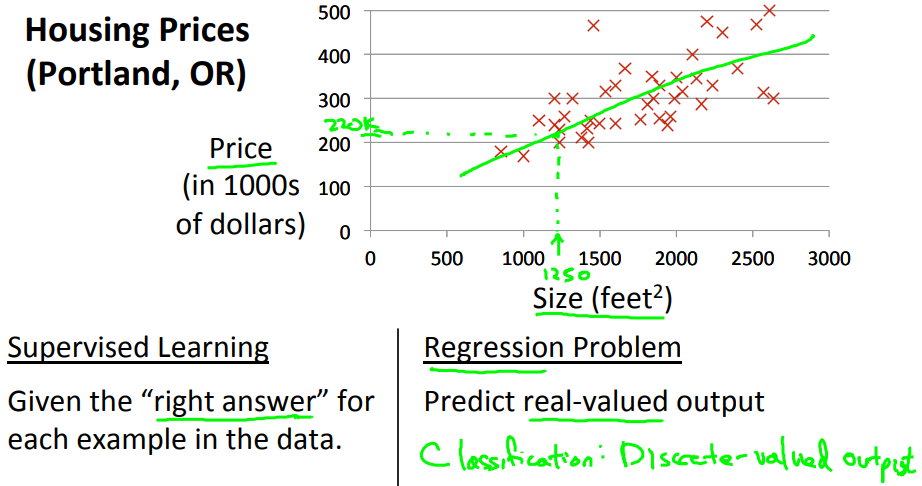
We're going to use a data set of housing prices from the city of Portland, Oregon. We plot my data set of a number of houses that were different sizes that were sold for a range of different prices.

Let's say that given this data set, you have a friend that's trying to sell a house and let's see if friend's house is size of 1250 square feet and you want to tell them how much they might be able to sell the house for.

Well one thing you could do is fit a straight line to this data.

Based on that, maybe you could tell your friend that let's say maybe he can sell the house for around $220,000. So this is an example of a supervised learning algorithm.

And it's supervised learning because we're given the, quotes, "right answer" for each of our examples. Namely we're told what was the actual house, what was the actual price of each of the houses in our data set were sold for and moreover, this is an example of a regression problem where the term regression refers to the fact that we are predicting a real-valued output namely the price.

And just to remind you the other most common type of supervised learning problem is called the classification problem where we predict discrete-valued outputs such as if we are looking at cancer tumors and trying to decide if a tumor is malignant or benign.

So that's a zero-one valued discrete output. More formally, in supervised learning, we have a data set and this data set is called a training set.

So for housing prices example, we have a training set of different housing prices and our job is to learn from this data how to predict prices of the houses.

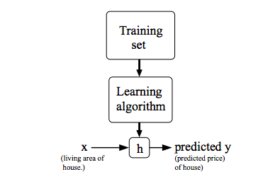
We saw that with the training set like our training set of housing prices and we feed that to our learning algorithm. Is the job of a learning algorithm to then output a function which by convention is usually denoted lowercase h and h stands for hypothesis

And what the job of the hypothesis is, is, is a function that takes as input the size of a house like maybe the size of the new house your friend's trying to sell so it takes in the value of x and it tries to output the estimated value of y for the corresponding house.

So h is a function that maps from x's to y's.

When designing a learning algorithm, the next thing we need to decide is how do we represent this hypothesis h and we will write this as \( h_\theta(x) = \theta_0 + \theta_1(x) \).

And plotting this in the pictures, all this means is that, we are going to predict that y is a linear function of x.

This model is called linear regression or this, for example, is actually linear regression with one variable, with the variable being x. Predicting all the prices as functions of one variable X. And another name for this model is univariate linear regression.

In linear progression, we have a training set that is showed below remember on notation M was the number of training examples, so m equals 47. And the form of our hypothesis,

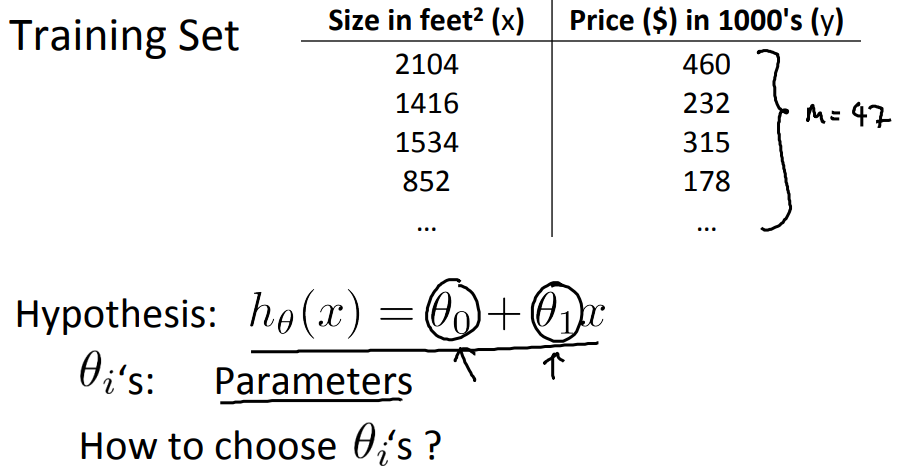
which we use to make predictions is this linear function. \( h_{\theta}(x) = \theta_0 + \theta_1(x) \)

These theta zero and theta one, they stabilize what I call the parameters of the model. Now next step is to go about choosing these two parameter values, theta 0 and theta 1.

With different choices of the parameter's theta 0 and theta 1, we get different hypothesis, different hypothesis functions s shown below.

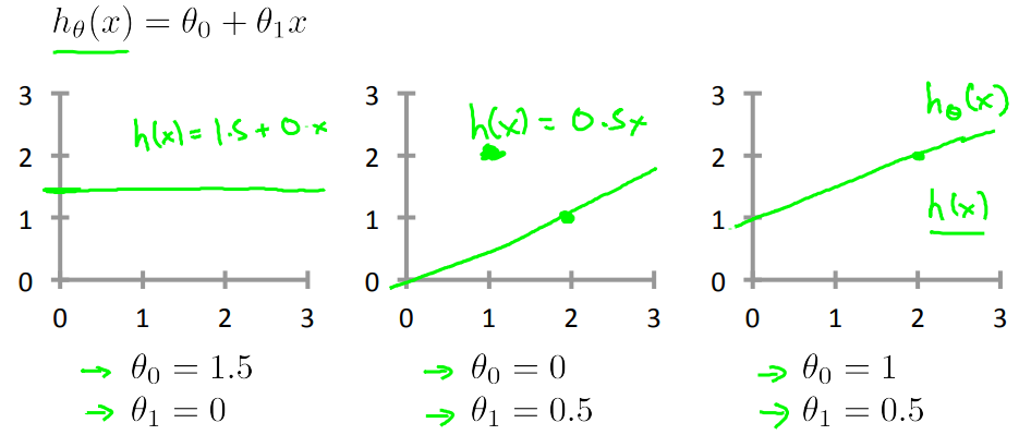
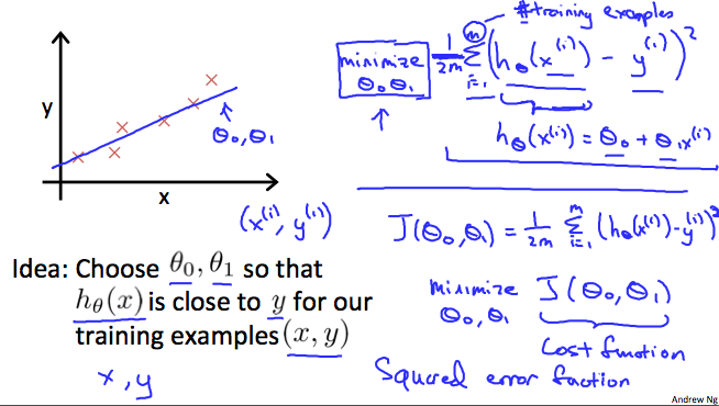
In linear regression, we have a training set, What we want to do, is come up with values for the parameters theta zero and theta one so that the straight line we get out of this, corresponds to a straight line that somehow fits the data well.

So, how do we come up with values, theta zero, theta one, that corresponds to a good fit to the data?

The idea is we get to choose our parameters theta 0, theta 1 so that h of x, meaning the value we predict on input x, that this is at least close to the values y for the examples in our training set, for our training examples.

So in our training set, we've given a number of examples where we know X decides the wholes and we know the actual price is was sold for. So, let's try to choose values for the parameters so that, at least in the training set, given the X in the training set we make reason of the active predictions for the Y values.

So linear regression, what we're going to do is, I'm going to want to solve a minimization problem.

\( \min_{\theta_0, \theta_1} \frac{1}{2m} \sum_{i = 1}^{m} (h_{\theta}(x_i) - y_i)^2 \)

Description of above equation :

Cost Function

If we try to think of it in visual terms, our training data set is scattered on the x-y plane. We are trying to make a straight line (defined by \( h_\theta(x) \) ) which passes through these scattered data points.

Our objective is to get the best possible line. The best possible line will be such so that the average squared vertical distances of the scattered points from the line will be the least. Ideally, the line should pass through all the points of our training data set. In such a case, the value of ( \(J(\theta_0, \theta_1) \) ) will be 0. The following example shows the ideal situation where we have a cost function of 0.

A simplified hypothesis function is just \( h(x) = \theta_1(x) \). We think of this as setting the parameter \( \theta_0 = 0 \) .

Using this simplified definition of a hypothesizing cost function let's try to understand the cost function concept better.

It turns out that two key functions we want to understand. The first is the hypothesis function, and the second is a cost function.

Let's plot these functions and try to understand them both better.

Let's start with the hypothesis. On the left, let's say here's my training set with three points at (1, 1), (2, 2), and (3, 3). Let's pick a value theta one, so when theta one equals one, and if that's my choice for theta one, then my hypothesis is going to look like this straight line over here.

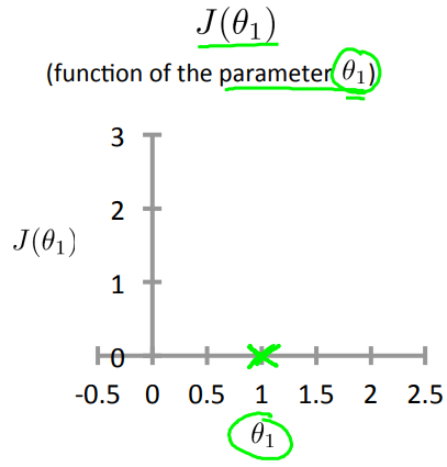
And I'm gonna point out, when I'm plotting my hypothesis function. X-axis, my horizontal axis is labeled X, is labeled you know, size of the house over here. Now, of temporary, set theta one equals one, what I want to do is figure out what is j of theta one, when theta one equals one. So let's go ahead and compute what the cost function has for.

\( J = \frac{1}{2m} \sum_{i=1}^{m} (h_{\theta}(x^{(i)}) - y^{(i)} )^2 \)

\( J = \frac{1}{2m} (0^2 + 0^2 + 0^2)^2 = 0 \)

Plotting \( J(\theta) \) with the parameter \( \theta_1 \)

When I plot different J for different \( \theta_1 \) we can get the below figure:

Right, so for each value of theta one we wound up with a different value of J of theta one and we could then use this to trace out this plot below.

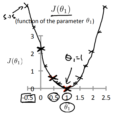
Now you remember, the optimization objective for our learning algorithm is we want to choose the value of theta one. That minimizes J of theta one.

This was our objective function for the linear regression. Well, looking at this curve, the value that minimizes j of theta one is, you know, theta one equals to one. And low and behold, that is indeed the best possible straight line fit through our data, by setting theta one equals one. And just, for this particular training set, we actually end up fitting it perfectly. And that's why minimizing j of theta one corresponds to finding a straight line that fits the data well.

For this problem we have :

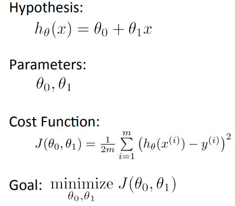
Hypothesis: \( h_{\theta}(x) = \theta_0 + \theta_1(x) \)
Parameters: \( \theta_0 , \theta_1 \)
Cost function : \( J(\theta_0 , \theta_1) = \frac{1}{2m} \sum_{i=1}^{m} (h_{\theta}(x^{(i)}) - y^{(i)})^2 \)
Goal : \( \min_{\theta_0 , \theta_1} J(\theta_0 , \theta_1) \)

The below figures shows a dataset with both variables \( \theta_0 , \theta_1 \), it also shows a special plot called contour plot that plot cost "J" against different values of the parameters \( \theta_0 , \theta_1 \)

A contour plot is a graph that contains many contour lines. A contour line of a two variable function has a constant value at all points of the same line. An example of such a graph is the one to the right below.

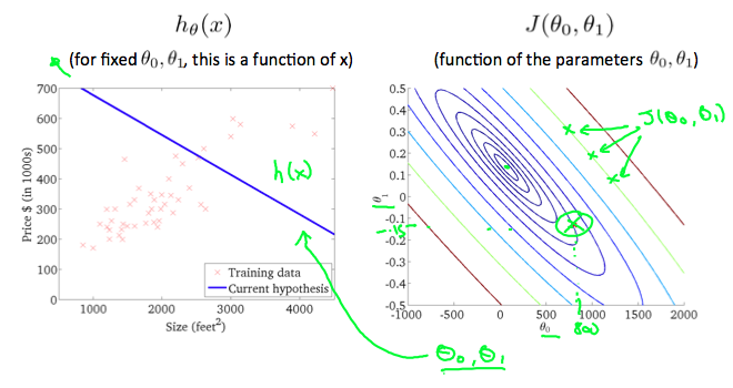
Taking any color and going along the 'circle', one would expect to get the same value of the cost function. For example, the three green points found on the green line above have the same value for \( J(\theta_0,\theta_1) \) and as a result, they are found along the same line. The circled x displays the value of the cost function for the graph on the left when \( \theta_0 = 800 \) and \( \theta_1 = -0.15 \). Taking another h(x) and plotting its contour plot, one gets the following graphs:

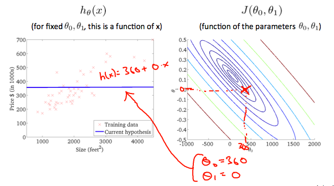
When \( \theta_0 = 360 \) and \( \theta_1 = 0 \) the value of \( J(\theta_0 , \theta_1) \) in the contour plot gets closer to the center thus reducing the cost function error. Now giving our hypothesis function a slightly positive slope results in a better fit of the data.

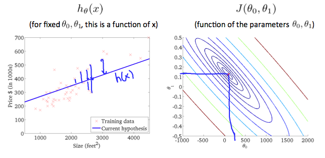
The graph above minimizes the cost function as much as possible and consequently, the result of \( \theta_0 \) and \( \theta_1 \) tend to be around 0.12 and 250 respectively. Plotting those values on our graph to the right seems to put our point in the center of the inner most 'circle'.