An algorithm called gradient descent is used for minimizing the cost function J. It turns out gradient descent is a more general algorithm, and is used not only in linear regression. It's actually used all over the place in machine learning.

And we'll use gradient descent to minimize other functions as well, not just the cost function J for the linear regression.

Here's the idea for gradient descent. What we're going to do is we're going to start off with some initial guesses for theta 0 and theta 1.

Doesn't really matter what they are, but a common choice would be we set theta 0 to 0, and set theta 1 to 0, just initialize them to 0.

What we're going to do in gradient descent is we'll keep changing theta 0 and theta 1 a little bit to try to reduce \( J(\theta_0, \theta_1) \), until hopefully, we wind at a minimum, or maybe at a local minimum.

So for linear regression we have our hypothesis function and we have a way of measuring how well it fits into the data. Now we need to estimate the parameters in the hypothesis function. That's where gradient descent comes in.

Imagine that we graph our hypothesis function based on its fields \( \theta_0 \) and \( \theta_1 \) (actually we are graphing the cost function as a function of the parameter estimates). We are not graphing x and y itself, but the parameter range of our hypothesis function and the cost resulting from selecting a particular set of parameters.

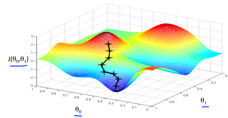
We put \( \theta_0 \) on the x axis and \( \theta_1 \) on the y axis, with the cost function on the vertical z axis. The points on our graph will be the result of the cost function using our hypothesis with those specific theta parameters. The graph above depicts such a setup.

We will know that we have succeeded when our cost function is at the very bottom of the pits in our graph, i.e. when its value is the minimum. The red arrows show the minimum points in the graph.

The way we do this is by taking the derivative (the tangential line to a function) of our cost function. The slope of the tangent is the derivative at that point and it will give us a direction to move towards. We make steps down the cost function in the direction with the steepest descent. The size of each step is determined by the parameter α, which is called the learning rate.

For example, the distance between each 'star' in the graph above represents a step determined by our parameter α. A smaller α would result in a smaller step and a larger α results in a larger step. The direction in which the step is taken is determined by the partial derivative of \( J(\theta_0,\theta_1) \). Depending on where one starts on the graph, one could end up at different points. The image above shows us two different starting points that end up in two different places.

Mathematically the definition of the gradient descent algorithm is given below .

We're going to just repeatedly do this until convergence, we're going to update my parameter theta j by taking theta j and subtracting from it alpha times this term over here.

First, this notation here, :=, gonna use := to denote assignment, so it's the assignment operator.

So briefly, if I write a := b, what this means is, it means in a computer, this means take the value in b and use it overwrite whatever value is a.

So this means set a to be equal to the value of b, which is assignment. And I can also do a := a + 1.

The alpha here is a number that is called the learning rate. And what alpha does is it basically controls how big a step we take downhill with creating descent. So if alpha is very large, then that corresponds to a very aggressive gradient descent procedure where we're trying take huge steps downhill and if alpha is very small, then we're taking little, little baby steps downhill.

This means take a and increase its value by one. Whereas in contrast, if I use the equal sign and I write a equals b, then this is a truth assertion.

repeat until convergence: \( \theta_j := \theta_j - \alpha \frac{\partial}{\partial \theta_j} J(\theta_0, \theta_1) \)

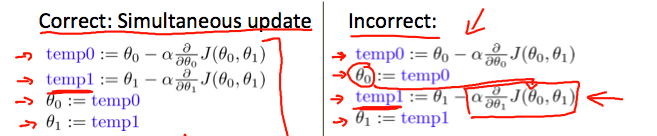
At each iteration j, one should simultaneously update the parameters \( \theta_1, \theta_2,...,\theta_n \) . Updating a specific parameter prior to calculating another one on the \( j^{(th)} \) iteration would yield to a wrong implementation.

where we used one parameter \( \theta_1 \) and plotted its cost function to implement a gradient descent. Our formula for a single parameter was :

Repeat until convergence:
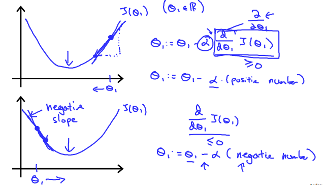
\( \theta_j := \theta_j - \alpha \frac{\partial}{\partial \theta_j} J(\theta_1) \)

Regardless of the slope's sign for \( \frac{d}{d\theta_1} J(\theta_1) \) eventually converges to its minimum value. The following graph shows that when the slope is negative, the value of \( \theta_1 \) increases and when it is positive, the value of \( \theta_1 \) decreases.

On a side note, we should adjust our parameter \( \alpha \) to ensure that the gradient descent algorithm converges in a reasonable time. Failure to converge or too much time to obtain the minimum value imply that our step size is wrong.

How does gradient descent converge with a fixed step size \( \alpha \)? The intuition behind the convergence is that \( \frac{d}{d\theta_1} J(\theta_1) \) approaches 0 as we approach the bottom of our convex function. At the minimum, the derivative will always be 0 and thus we get: \( \theta_1:=\theta_1-\alpha * 0 \)

When specifically applied to the case of linear regression, a new form of the gradient descent equation can be derived. We can substitute our actual cost function and our actual hypothesis function and modify the equation to :

\( \begin{align*} \text{repeat until convergence: } \lbrace & \newline \theta_0 := & \theta_0 - \alpha \frac{1}{m} \sum\limits_{i=1}^{m}(h_\theta(x_{i}) - y_{i}) \newline \theta_1 := & \theta_1 - \alpha \frac{1}{m} \sum\limits_{i=1}^{m}\left((h_\theta(x_{i}) - y_{i}) x_{i}\right) \newline \rbrace& \end{align*} \)

where m is the size of the training set, \( \theta_0 \) a constant that will be changing simultaneously with \( \theta_1 \) and \( x_{i}, y_{i} \) are values of the given training set (data).

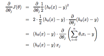
Note that we have separated out the two cases for \( \theta_j \) into separate equations for \( \theta_0 \) and \( \theta_1 \) and that for \( \theta_1 \) we are multiplying \( x_{i} \) at the end due to the derivative. The following is a derivation of \( \frac {\partial}{\partial \theta_j}J(\theta) \) for a single example :

The point of all this is that if we start with a guess for our hypothesis and then repeatedly apply these gradient descent equations, our hypothesis will become more and more accurate.

So, this is simply gradient descent on the original cost function J. This method looks at every example in the entire training set on every step, and is called batch gradient descent.

Note that, while gradient descent can be susceptible to local minima in general, the optimization problem we have posed here for linear regression has only one global, and no other local, optima; thus gradient descent always converges (assuming the learning rate α is not too large) to the global minimum.

Indeed, J is a convex quadratic function. Here is an example of gradient descent as it is run to minimize a quadratic function.

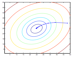
The ellipses shown above are the contours of a quadratic function. Also shown is the trajectory taken by gradient descent, which was initialized at (48,30).

The x’s in the figure (joined by straight lines) mark the successive values of θ that gradient descent went through as it converged to its minimum.