A new version of linear regression that's more powerful is one that works with multiple variables or with multiple features.

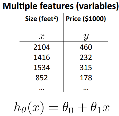
In the original version of linear regression that we developed in previous chapters, we have a single feature x, the size of the house, and we wanted to use that to predict why the price of the house and this was our form of our hypothesis.

But now imagine, what if we had not only the size of the house as a feature or as a variable of which to try to predict the price, but that we also knew the number of bedrooms, the number of house and the age of the home and years. It seems like this would give us a lot more information with which to predict the price.

To introduce a little bit of notation, we sort of started to talk about this earlier, I'm going to use the variables \( x_1, x_2 \) and so on to denote my, in this case, four features and I'm going to continue to use Y to denote the variable, the output variable price that we're trying to predict.

Now that we have four features we are going to use lowercase "n" to denote the number of features. So in this example we have n = 4 because we have four features.

And "n" is different from our earlier notation where we were using "n" to denote the number of examples. So if you have 47 rows "M" is the number of rows on this table or the number of training examples.

So I'm also going to use \( x^{(i)} \) to denote the input features of the "I" training example.

As a concrete example let say \( x_2 \) is going to be a vector of the features for my second training example. And so \( X_2 \) here is going to be a vector 1416, 3, 2, 40 since those are my four features that I have to try to predict the price of the second house.

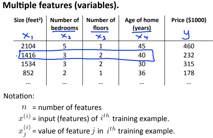
With this notation \( x_2 \) is a four dimensional vector. In fact, more generally, this is an n-dimensional feature back there. With this notation, \( x_2 \) is now a vector and so, I'm going to use also \( x_j^i \) to denote the value of feature number J and the ith training example. So \( x_{(3)}^2 \) is going to be equal to 2 as seen in the above figure.

Now that we have multiple features, let's talk about what the form of our hypothesis should be. Previously this was the form of our hypothesis, where x was our single feature, but now that we have multiple features, we aren't going to use the simple representation any more.

Instead, a form of the hypothesis in linear regression is going to be this, can be \( h_{\theta}(x) = \theta_0 + \theta_1 x_1 + \theta_2 x_2 + \theta_3 x_3 + ... + \theta_n x_n\). And if we have N features then rather than summing up over our four features, we would have a sum over our N features.

For convenience of notation, let me define \( x_0 \) to be equals one. Concretely, this means that for every example i, I have a feature vector \( X_i \) and \( x^i_{(0)} \) is going to be equal to 1. You can think of this as defining an additional zero feature. So now my feature vector X becomes this n+1 dimensional vector.

Using the definition of matrix multiplication, our multivariable hypothesis function can be concisely represented as:

\begin{align*}h_\theta(x) =\begin{bmatrix}\theta_0 \hspace{2em} \theta_1 \hspace{2em} ... \hspace{2em} \theta_n\end{bmatrix}\begin{bmatrix}x_0 \newline x_1 \newline \vdots \newline x_n\end{bmatrix}= \theta^T x\end{align*}

Which gives us \( \theta^T x = h_{\theta}(x) = \theta_0 + \theta_1 x_1 + \theta_2 x_2 + \theta_3 x_3 + ... + \theta_n x_n \)

Linear regression with multiple variables is also known as "multivariate linear regression".

We now introduce notation for equations where we can have any number of input variables.

\begin{align*}x_j^{(i)} &= \text{value of feature } j \text{ in the }i^{th}\text{ training example} \newline x^{(i)}& = \text{the input (features) of the }i^{th}\text{ training example} \newline m &= \text{the number of training examples} \newline n &= \text{the number of features} \end{align*}

The multivariable form of the hypothesis function accommodating these multiple features is as follows:

\( h_{\theta}(x) = \theta_0 + \theta_1 x_1 + \theta_2 x_2 + \theta_3 x_3 + ... + \theta_n x_n\)

In order to develop intuition about this function, we can think about \( \theta_0 \) as the basic price of a house, \( \theta_1 \) as the price per square meter, \( \theta_2 \) as the price per floor, etc. \( x_1 \) will be the number of square meters in the house, \( x_2 \) the number of floors, etc.

Using the definition of matrix multiplication, our multivariable hypothesis function can be concisely represented as:

\begin{align*}h_\theta(x) =\begin{bmatrix}\theta_0 \hspace{2em} \theta_1 \hspace{2em} ... \hspace{2em} \theta_n\end{bmatrix}\begin{bmatrix}x_0 \newline x_1 \newline \vdots \newline x_n\end{bmatrix}= \theta^T x\end{align*}

This is a vectorization of our hypothesis function for one training example; see the lessons on vectorization to learn more.

Remark: Note that for convenience reasons in this course we assume \( x_{0}^{(i)} = 1 \text{ for } (i\in { 1,\dots, m } \) This allows us to do matrix operations with theta and x. Hence making the two vectors \( '\theta' \) and \( x^{(i)} \) match each other element-wise (that is, have the same number of elements: n+1).