To attempt classification, one method is to use linear regression and map all predictions greater than 0.5 as a 1 and all less than 0.5 as a 0. However, this method doesn't work well because classification is not actually a linear function.

The classification problem is just like the regression problem, except that the values we now want to predict take on only a small number of discrete values.

For now, we will focus on the binary classification problem in which y can take on only two values, 0 and 1. (Most of what we say here will also generalize to the multiple-class case.)

For instance, if we are trying to build a spam classifier for email, then \( x^{(i)} \) may be some features of a piece of email, and y may be 1 if it is a piece of spam mail, and 0 otherwise. Hence, \( y \in {0,1} \).

0 is also called the negative class, and 1 the positive class, and they are sometimes also denoted by the symbols “-” and “+.” Given \( x^{(i)} \) , the corresponding \( y^{(i)} \) is also called the label for the training example.

Earlier we talked about email spam classification as an example of a classification problem. Another example would be classifying online transactions.

So if you have a website that sells stuff and if you want to know if a particular transaction is fraudulent or not, whether someone is using a stolen credit card or has stolen the user's password.

There's another classification problem. And earlier we also talked about the example of classifying tumors as cancerous, malignant or as benign tumors.

In all of these problems the variable that we're trying to predict is a variable 'y' that we can think of as taking on two values either zero or one, either spam or not spam, fraudulent or not fraudulent, related malignant or benign.

Another name for the class that we denote with zero is the negative class, and another name for the class that we denote with one is the positive class. So zero we denote as the benign tumor, and one, positive class we denote a malignant tumor.

The assignment of the two classes, spam not spam and so on. The assignment of the two classes to positive and negative to zero and one is somewhat arbitrary and it doesn't really matter but often there is this intuition that a negative class is conveying the absence of something like the absence of a malignant tumor.

Whereas one the positive class is conveying the presence of something that we may be looking for, but the definition of which is negative and which is positive is somewhat arbitrary and it doesn't matter that much.

For now we're going to start with classification problems with just two classes zero and one. Later one we'll talk about multi class problems as well where therefore y may take on four values zero, one, two, and three.

This is called a multiclass classification problem.

Here's an example of a training set for a classification task for classifying a tumor as malignant or benign. And notice that malignancy takes on only two values, zero or no, one or yes. So one thing we could do given this training set is to apply the algorithm that we already know.

Linear regression to this data set and just try to fit the straight line to the data. So if you take this training set and fill a straight line to it, maybe you get a hypothesis.

If you want to make predictions one thing you could try doing is then threshold the classifier outputs at 0.5 that is at a vertical axis value 0.5 and if the hypothesis outputs a value that is greater than equal to 0.5 you can take y = 1.

If it's less than 0.5 you can take y=0. So 0.5 and so that's where the threshold is and that's using linear regression this way. Everything to the right of this point we will end up predicting as the positive cross. Because the output values is greater than 0.5 on the vertical axis and everything to the left of that point we will end up predicting as a negative value.

If we were to use linear regression for a classification problem. For classification we know that y is either zero or one. But if you are using linear regression where the hypothesis can output values that are much larger than one or less than zero, even if all of your training examples have labels y equals zero or one.

So we develop an algorithm called logistic regression, which has the property that the output, the predictions of logistic regression are always between zero and one, and doesn't become bigger than one or become less than zero.

What is the function we're going to use to represent our hypothesis when we have a classification problem?

We could approach the classification problem ignoring the fact that y is discrete-valued, and use our old linear regression algorithm to try to predict y given x.

However, it is easy to construct examples where this method performs very poorly. Intuitively, it also doesn’t make sense for \( h_{\theta}(x)\) to take values larger than 1 or smaller than 0 when we know that \( y \in {0, 1} \).

To fix this, let’s change the form for our hypotheses \( h_{\theta}(x) \) to satisfy \( 0 \leq h_\theta (x) \leq 1 \). This is accomplished by plugging \( \theta^Tx \) into the Logistic Function.

Our new form uses the "Sigmoid Function," also called the "Logistic Function":

\( \begin{align*}& h_\theta (x) = g ( \theta^T x ) \newline \newline& z = \theta^T x \newline& g(z) = \dfrac{1}{1 + e^{-z}}\end{align*} \)

The following image shows us what the sigmoid function looks like:

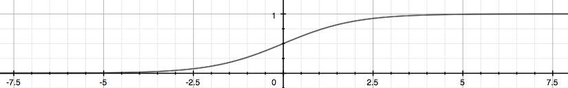
The function g(z), shown here, maps any real number to the (0, 1) interval, making it useful for transforming an arbitrary-valued function into a function better suited for classification.

\( h_\theta(x) \) will give us the probability that our output is 1. For example, \( h_\theta(x) = 0.7 \) gives us a probability of 70% that our output is 1. Our probability that our prediction is 0 is just the complement of our probability that it is 1 (e.g. if probability that it is 1 is 70%, then the probability that it is 0 is 30%).

\( \begin{align*}& h_\theta(x) = P(y=1 | x ; \theta) = 1 - P(y=0 | x ; \theta) \newline& P(y = 0 | x;\theta) + P(y = 1 | x ; \theta) = 1\end{align*} \)

We may have a feature vector x, which is this x zero equals one as always. And then one feature is the size of the tumor.

Suppose a patient comes in and they have some tumor size and we feed their feature vector x into the hypothesis. And suppose the hypothesis outputs the number 0.7.

I'm going to interpret my hypothesis as follows. I'm gonna say that this hypothesis is telling me that for a patient with features x, the probability that y equals 1 is 0.7. In other words, I'm going to tell my patient that the tumor, sadly, has a 70 percent chance, or a 0.7 chance of being malignant.

To write this out more formally as: \( P(y = 1 | x ; \theta) \)

Here's how I read this expression. This is the probability that y is equal to one. Given x, given that my patient has features x, so given my patient has a particular tumor size represented by my features x. And this probability is parameterized by theta.

Similarly \( P(y = 0 | x ; \theta) \) is saying that probability of y=0 for a particular patient with features x, and given our parameters theta.

We no that probabilities add up to one so : \( P(y = 0 | x ; \theta) + P(y = 1 | x ; \theta) = 1 \)

In order to get our discrete 0 or 1 classification, we can translate the output of the hypothesis function as follows:

\( \begin{align*}& h_\theta(x) \geq 0.5 \rightarrow y = 1 \newline& h_\theta(x) < 0.5 \rightarrow y = 0 \newline\end{align*} \)

The way our logistic function g behaves is that when its input is greater than or equal to zero, its output is greater than or equal to 0.5:

\( \begin{align*}& g(z) \geq 0.5 \newline& when \; z \geq 0\end{align*} \)

Remember.

\( \begin{align*}z=0, e^{0}=1 \Rightarrow g(z)=1/2\newline z \to \infty, e^{-\infty} \to 0 \Rightarrow g(z)=1 \newline z \to -\infty, e^{\infty}\to \infty \Rightarrow g(z)=0 \end{align*} \)

So if our input to g is \( \theta^T X \), then that means:

\( \begin{align*}& h_\theta(x) = g(\theta^T x) \geq 0.5 \newline& when \; \theta^T x \geq 0\end{align*} \)

From these statements we can now say:

\( \begin{align*}& \theta^T x \geq 0 \Rightarrow y = 1 \newline& \theta^T x < 0 \Rightarrow y = 0 \newline\end{align*} \)

The decision boundary is the line that separates the area where y = 0 and where y = 1. It is created by our hypothesis function.

Example:

\( \begin{align*}& \theta = \begin{bmatrix}5 \newline -1 \newline 0\end{bmatrix} \newline & y = 1 \; if \; 5 + (-1) x_1 + 0 x_2 \geq 0 \newline & 5 - x_1 \geq 0 \newline & - x_1 \geq -5 \newline& x_1 \leq 5 \newline \end{align*} \)

In this case, our decision boundary is a straight vertical line placed on the graph where \( x_1 = 5 \), and everything to the left of that denotes y = 1, while everything to the right denotes y = 0.

Again, the input to the sigmoid function g(z) (e.g. \( \theta^T X \) doesn't need to be linear, and could be a function that describes a circle (e.g. \( z = \theta_0 + \theta_1 x_1^2 +\theta_2 x_2^2 \) ) or any shape to fit our data.