We cannot use the same cost function that we use for linear regression because the Logistic Function will cause the output to be wavy, causing many local optima. In other words, it will not be a convex function.

Instead, our cost function for logistic regression looks like:

\( \begin{align*}& J(\theta) = \dfrac{1}{m} \sum_{i=1}^m \mathrm{Cost}(h_\theta(x^{(i)}),y^{(i)}) \newline & \mathrm{Cost}(h_\theta(x),y) = -\log(h_\theta(x)) \; & \text{if y = 1} \newline & \mathrm{Cost}(h_\theta(x),y) = -\log(1-h_\theta(x)) \; & \text{if y = 0}\end{align*} \)

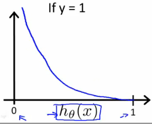
When y = 1, we get the following plot for \( J(\theta) v. h_\theta (x) \):

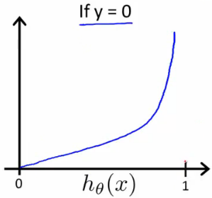
Similarly, when y = 0, we get the following plot for \( J(\theta) v. h_\theta (x) \):

\( \begin{align*}& \mathrm{Cost}(h_\theta(x),y) = 0 \text{ if } h_\theta(x) = y \newline & \mathrm{Cost}(h_\theta(x),y) \rightarrow \infty \text{ if } y = 0 \; \mathrm{and} \; h_\theta(x) \rightarrow 1 \newline & \mathrm{Cost}(h_\theta(x),y) \rightarrow \infty \text{ if } y = 1 \; \mathrm{and} \; h_\theta(x) \rightarrow 0 \newline \end{align*} \)

If our correct answer 'y' is 0, then the cost function will be 0 if our hypothesis function also outputs 0. If our hypothesis approaches 1, then the cost function will approach infinity.

If our correct answer 'y' is 1, then the cost function will be 0 if our hypothesis function outputs 1. If our hypothesis approaches 0, then the cost function will approach infinity.

Note that writing the cost function in this way guarantees that J(θ) is convex for logistic regression.

We can compress our cost function's two conditional cases into one case:

\( Cost(h_{\theta}(x),y)=−ylog(h_{\theta}(x))−(1−y)log(1−h_{\theta}(x)) \)

Notice that when y is equal to 1, then the second term \( (1-y)\log(1-h_\theta(x)) \) will be zero and will not affect the result. If y is equal to 0, then the first term \( -y \log(h_\theta(x)) \) will be zero and will not affect the result.

We can fully write out our entire cost function as follows:

\( J(\theta) = − \frac{1}{m} \sum_{i = 1}^{m} [y^{(i)}log(h_{\theta}(x^{(i)}))−(1−y^{(i)})log(1−h_{\theta}(x^{(i)})) ] \)

A vectorized implementation is:

\begin{align*} & h = g(X\theta)\newline & J(\theta) = \frac{1}{m} \cdot \left(-y^{T}\log(h)-(1-y)^{T}\log(1-h)\right) \end{align*}

Gradient Descent:

"Conjugate gradient", "BFGS", and "L-BFGS" are more sophisticated, faster ways to optimize θ that can be used instead of gradient descent. We suggest that you should not write these more sophisticated algorithms yourself (unless you are an expert in numerical computing) but use the libraries instead, as they're already tested and highly optimized. Octave provides them.

We first need to provide a function that evaluates the following two functions for a given input value θ:

\begin{align*} & J(\theta) \newline & \dfrac{\partial}{\partial \theta_j}J(\theta)\end{align*}

We can write a single function that returns both of these:

function [jVal, gradient] = costFunction(theta)
  jVal = [...code to compute J(theta)...];
  gradient = [...code to compute derivative of J(theta)...];
end

Then we can use octave's "fminunc()" optimization algorithm along with the "optimset()" function that creates an object containing the options we want to send to "fminunc()".

options = optimset('GradObj', 'on', 'MaxIter', 100);
initialTheta = zeros(2,1);
   [optTheta, functionVal, exitFlag] = fminunc(@costFunction, initialTheta, options);

We give to the function "fminunc()" our cost function, our initial vector of theta values, and the "options" object that we created beforehand.

Now we will approach the classification of data when we have more than two categories. Instead of y = {0,1} we will expand our definition so that y = {0,1...n}.

Since y = {0,1...n}, we divide our problem into n+1 (+1 because the index starts at 0) binary classification problems; in each one, we predict the probability that 'y' is a member of one of our classes.

\( \begin{align*}& y \in \lbrace0, 1 ... n\rbrace \newline& h_\theta^{(0)}(x) = P(y = 0 | x ; \theta) \newline& h_\theta^{(1)}(x) = P(y = 1 | x ; \theta) \newline& \cdots \newline& h_\theta^{(n)}(x) = P(y = n | x ; \theta) \newline& \mathrm{prediction} = \max_i( h_\theta ^{(i)}(x) )\newline\end{align*} \)

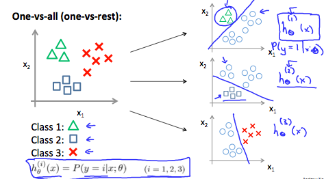
We are basically choosing one class and then lumping all the others into a single second class. We do this repeatedly, applying binary logistic regression to each case, and then use the hypothesis that returned the highest value as our prediction.

The following image shows how one could classify 3 classes:

To summarize: