Standard Deviation
The two measures of spread; the range (covered by all the data) and the inter-quartile range (IQR), which looks at the range covered by the middle 50% of the distribution. We noted that the IQR should be paired as a measure of spread with the median as a measure of center
The standard deviation, which quantifies the spread of a distribution in a completely different way
The idea behind the standard deviation is to quantify the spread of a distribution by measuring how far the observations are from their mean, \( \overline{x} \) . The standard deviation gives the average (or typical distance) between a data point and the mean, \( \overline{x} \).
There are many notations for the standard deviation: SD, s, Sd, StDev. Here, we'll use SD as an abbreviation for standard deviation, and use s as the symbol.
In order to get a better understanding of the standard deviation, it would be useful to see an example of how it is calculated.
The following are the number of customers who entered a video store in 8 consecutive hours: 7, 9, 5, 13, 3, 11, 15, 9
To find the standard deviation of the number of hourly customers: Find the mean, \( \overline{x} \) of your data : \( \frac{7 + 9 + 5 + 13 + 3 + 11 + 15 + 9}{8} = 9\)
Find the deviations from the mean: the difference between each observation and the mean (7 - 9), (9 - 9), (5 - 9), (13 - 9), (3 - 9), (11 - 9), (15 - 9), (9 - 9) = -2, 0, -4, 4, -6, 2, 6, 0 Since the standard deviation is the average (typical) distance between the data points and their mean, it would make sense to average the deviations we got. Note, however, that the sum of the deviations from the mean, is 0 (add them up and see for yourself). This is always the case, and is the reason why we have to do a more complicated calculation to determine the standard deviation
Square each of the deviations: Average the square deviations by adding them up, and dividing by n - 1, (one less than the sample size) the reason why we "sort of" average the square deviations (divide by n - 1) rather than take the actual average (divide by n) is beyond the scope of the course at this point, but will be addressed later. This average of the squared deviations is called the variance of the data.
The SD of the data is the square root of the variance: SD = \( \sqrt{16} = 4 \)
Why do we take the square root? Note that 16 is an average of the squared deviations, and therefore has different units of measurement. In this case 16 is measured in "squared customers," which obviously cannot be interpreted. We therefore take the square root in order to compensate for the fact that we squared our deviations, and in order to go back to the original unit of measurement. Recall that the average number of customers who enter the store in an hour is 9. The interpretation of SD = 4 is that on average, the actual number of customers that enter the store each hour is 4 away from 9.
Properties of the Standard Deviation
It should be clear from the discussion thus far that the SD should be paired as a measure of spread with the mean as a measure of center.
Note that the only way, mathematically, in which the SD = 0, is when all the observations have the same value (Ex: 5, 5, 5, ... , 5), in which case, the deviations from the mean (which is also 5) are all 0. This is intuitive, since if all the data points have the same value, we have no variability (spread) in the data, and expect the measure of spread (like the SD) to be 0. Indeed, in this case, not only is the SD equal to 0, but the range and the IQR are also equal to 0.
Like the mean, the SD is strongly influenced by outliers in the data. Consider the example where: 3, 5, 7, 9, 9, 11, 13, 15 (data ordered). If the largest observation was wrongly recorded as 150, then the average would jump up to 25.9, and the standard deviation would jump up to SD = 50.3. Note that in this simple example, it is easy to see that while the standard deviation is strongly influenced by outliers, the IQR is not. The IQR would be the same in both cases, since, like the median, the calculation of the quartiles depends only on the order of the data rather than the actual values.
The last comment leads to the following very important conclusion:
Choosing Numerical Summaries
Use (the mean) and the standard deviation as measures of center and spread only for reasonably symmetric distributions with no outliers.
Use the five-number summary (which gives the median, IQR and range) for all other cases
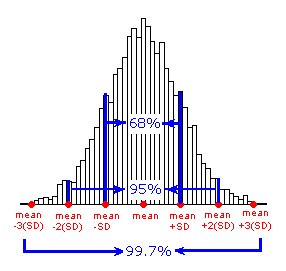
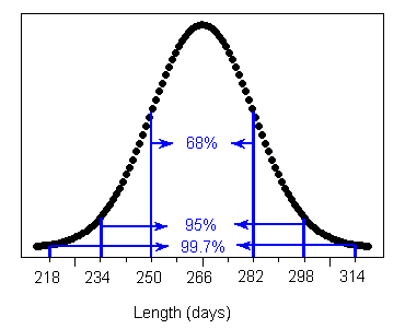
Standard Deviation Rule / The Empirical Rule
Consider a symmetric mound-shaped distribution: For distributions having this shape (also known as the normal shape), the following rule applies:
The Standard Deviation Rule:
Approximately 68% of the observations fall within 1 standard deviation of the mean.
Approximately 95% of the observations fall within 2 standard deviations of the mean.
Approximately 99.7% (or virtually all) of the observations fall within 3 standard deviations of the mean.
The following picture illustrates this rule:
This rule provides another way to interpret the standard deviation of a distribution, and thus also provides a bit more intuition about it.
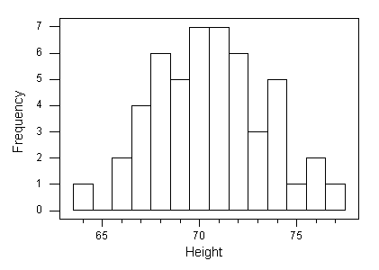
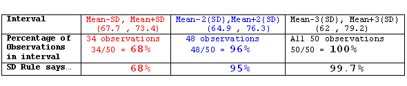
The following histogram represents height (in inches) of 50 males. Note that the data are roughly normal, so we would like to see how the Standard Deviation Rule works for this example.
Below are the actual data, and the numerical summaries of the distribution. Note that the key players here, the mean and standard deviation, have been highlighted.
To see how well the Standard Deviation Rule works for this case, we will find what percentage of the observations falls within 1, 2, and 3 standard deviations from the mean, and compare it to what the Standard Deviation Rule tells us this percentage should be.
It turns out the Standard Deviation Rule works very well in this example.
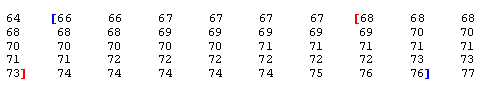
| Statistic | Height |
|---|---|
| N | 50 |
| Mean | 70.58 |
| StDev | 2.858 |
| min | 64 |
| Q1 | 68 |
| Median | 70.5 |
| Q3 | 72 |
| Max | 77 |
Standard Deviation Rule: Applications
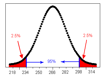
Example: Length of Human Pregnancy : The length of the human pregnancy is not fixed. It is known that it varies according to a distribution which is roughly normal, with a mean of 266 days, and a standard deviation of 16 days.
We can now use the information provided by the Standard Deviation Rule about the distribution of the length of human pregnancy, to answer some questions. For example : Question: How long do the middle 95% of human pregnancies last? Answer: The middle 95% of pregnancies last within 2 standard deviations of the mean, or in this case 234-298 days.
Question: What percent of pregnancies last more than 298 days? Since 95% of the pregnancies last between 234 and 298 days, the remaining 5% of pregnancies last either less than 234 days or more than 298 days. Since the normal distribution is symmetric, these 5% of pregnancies are divided evenly between the two tails, and therefore 2.5% of pregnancies last more than 298 days.
Question: How short are the shortest 2.5% of pregnancies? Using the same reasoning as in the previous question, the shortest 2.5% of human pregnancies last less than 234 days.
Question: What percent of human pregnancies last more than 266 days? Since 266 days is the mean, approximately 50% of pregnancies last more than 266 days.
Standard Deviation Rule: Applications
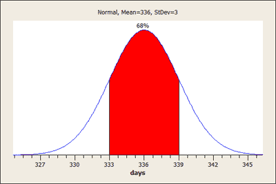
Q . Almost all (99.7%) horse pregnancies fall in what range of lengths? Between 327 and 345 days. The Standard Deviation Rule tells us that virtually all the data fall within 3 standard deviations of the mean, which in this case is exactly between 336 - 3(3) = 327, and 336 + 3(3) = 345.
Q. What percentage of horse pregnancies last longer than 339 days? 16% . According to the SD rule, 68% of horse pregnancies last between 336 - 3 = 333 and 336 + 3 = 339 days, which means that the remaining 32% of horse pregnancies are divided evenly between lasting less than 333 days and lasting more than 339 days. We therefore conclude that 16% of horse pregnancies last more than 339 days.
Standard Deviation Rule: Applications
The standard deviation measures the spread by reporting a typical (average) distance between the data points and their average
It is appropriate to use the SD as a measure of spread with the mean as the measure of center.
Since the mean and standard deviations are highly influenced by extreme observations, they should be used as numerical descriptions of the center and spread only for distributions that are roughly symmetric, and have no outliers. For symmetric mound-shaped distributions, the Standard Deviation Rule tells us what percentage of the observations falls within 1, 2, and 3 standard deviations of the mean, and thus provides another way to interpret the standard deviation's value for distributions of this type.