Diagnosing Bias vs. Variance
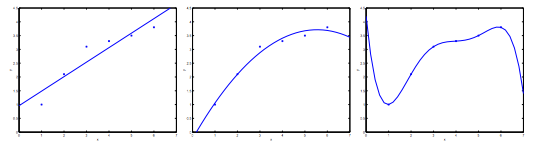
In this section we examine the relationship between the degree of the polynomial d and the underfitting or overfitting of our hypothesis.
We need to distinguish whether bias or variance is the problem contributing to bad predictions.
High bias is underfitting and high variance is overfitting. Ideally, we need to find a golden mean between these two.
The training error will tend to decrease as we increase the degree d of the polynomial.
At the same time, the cross validation error will tend to decrease as we increase d up to a point, and then it will increase as d is increased, forming a convex curve.
High bias (underfitting): both \( J_{train}(\Theta) \) and \( J_{CV}(\Theta) \) will be high. Also, \( J_{CV}(\Theta) \approx J_{train}(\Theta) \).
High variance (overfitting): \( J_{train}(\Theta) \) will be low and \( J_{CV}(\Theta) \) will be much greater than \( J_{train}(\Theta) \).
The is summarized in the figure below:
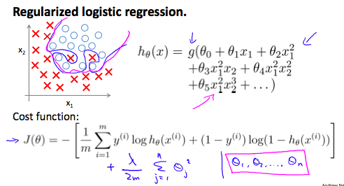
Regularization and Bias/Variance
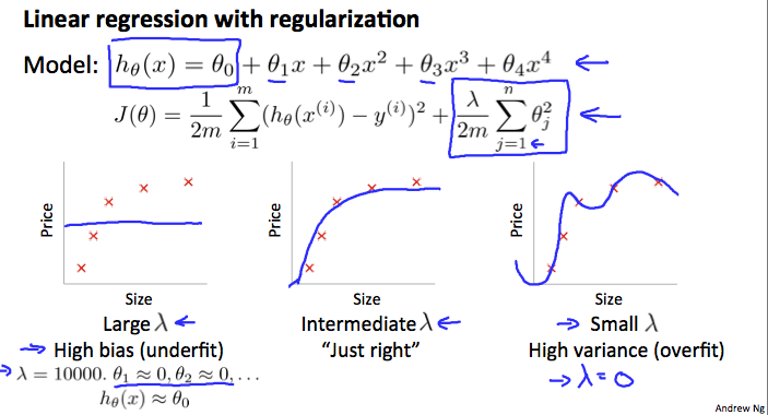
In the figure above, we see that as \( \lambda \) increases, our fit becomes more rigid.
On the other hand, as \( \lambda \) approaches 0, we tend to over overfit the data.
So how do we choose our parameter \( \lambda \) to get it 'just right' ? In order to choose the model and the regularization term λ, we need to:
Create a list of lambdas (i.e. λ ∈ {0,0.01,0.02,0.04,0.08,0.16,0.32,0.64,1.28,2.56,5.12,10.24});
Create a set of models with different degrees or any other variants.
Iterate through the \( \lambda \) and for each \( \lambda \) go through all the models to learn some \( \Theta \).
Compute the cross validation error using the learned Θ (computed with λ) on the \( J_{CV}(\Theta) \) without regularization or λ = 0.
Select the best combo that produces the lowest error on the cross validation set.
Using the best combo Θ and λ, apply it on \( J_{test}(\Theta) \) to see if it has a good generalization of the problem.
Learning Curves
Training an algorithm on a very few number of data points (such as 1, 2 or 3) will easily have 0 errors because we can always find a quadratic curve that touches exactly those number of points. Hence:
As the training set gets larger, the error for a quadratic function increases.
The error value will plateau out after a certain m, or training set size. Experiencing high bias:
Low training set size: causes \( J_{train}(\Theta) \) to be low and \( J_{CV}(\Theta) \) to be high.
Large training set size: causes both \( J_{train}(\Theta) \) and \( J_{CV}(\Theta) \) to be high with \( J_{train}(\Theta) \sim J_{CV}(\Theta) \).
If a learning algorithm is suffering from high bias, getting more training data will not (by itself) help much.
Experiencing high variance:
Low training set size: \( J_{train}(\Theta) \) will be low and \( J_{CV}(\Theta) \) will be high.
Large training set size: \( J_{train}(\Theta) \) increases with training set size and \( J_{CV}(\Theta) \) continues to decrease without leveling off. Also, \( J_{train}(\Theta) < J_{CV}(\Theta) \) but the difference between them remains significant.
If a learning algorithm is suffering from high variance, getting more training data is likely to help.
Deciding What to Do Next
Our decision process can be broken down as follows:
Getting more training examples: Fixes high variance
Trying smaller sets of features: Fixes high variance
Adding features: Fixes high bias
Adding polynomial features: Fixes high bias
Decreasing λ: Fixes high bias
Increasing λ: Fixes high variance.
Diagnosing Neural Networks
A neural network with fewer parameters is prone to underfitting. It is also computationally cheaper.
A large neural network with more parameters is prone to overfitting. It is also computationally expensive. In this case you can use regularization (increase λ) to address the overfitting.
Using a single hidden layer is a good starting default.
You can train your neural network on a number of hidden layers using your cross validation set. You can then select the one that performs best.
Model Complexity Effects:
Lower-order polynomials (low model complexity) have high bias and low variance.
In this case, the model fits poorly consistently.
Higher-order polynomials (high model complexity) fit the training data extremely well and the test data extremely poorly.
These have low bias on the training data, but very high variance.
In reality, we would want to choose a model somewhere in between, that can generalize well but also fits the data reasonably well.