Optimization Objective
With supervised learning, the performance of many supervised learning algorithms will be pretty similar, and what matters less often will be whether you use learning algorithm a or learning algorithm b, but what matters more will often be things like the amount of data you create these algorithms on, as well as your skill in applying these algorithms.
Things like your choice of the features you design to give to the learning algorithms, and how you choose the regularization parameter, and things like that.
But, there's one more algorithm that is very powerful and is very widely used both within industry and academia, and that's called the support vector machine.
And compared to both logistic regression and neural networks, the Support Vector Machine, or SVM sometimes gives a cleaner, and sometimes more powerful way of learning complex non-linear functions.
In order to describe the support vector machine, we are going to start with logistic regression, and show how we can modify it a bit, and get what is essentially the support vector machine.
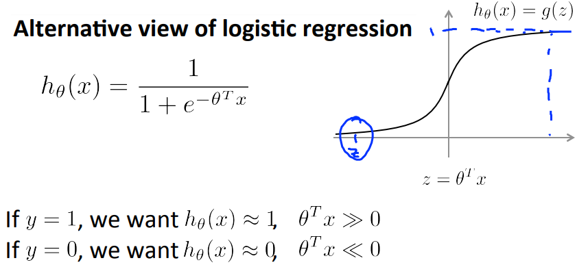
In logistic regression, we have our familiar form of the hypothesis there and the sigmoid activation function shown on the right.
In logistic regression if we have an example with y equals one then \( h_\theta(x) \sim 1 \). This means that \( \theta x >> 0 \). Conversely, if we have an example where y is equal to zero, \( h_\theta(x) \sim 0 \). This means that \( \theta x << 0 \)
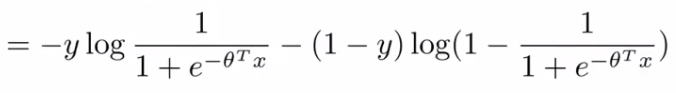
If you look at the cost function of logistic regression, you'll find is that each example (x,y) contributes a term given below to the overall cost function.

For the overall cost function, we sum over all the training examples using the above function, and have a 1/m term If you then plug in the hypothesis definition (hθ(x)), you get an expanded cost function equation;
So each training example contributes that term to the cost function for logistic regression. If y = 1 then only the first term in the objective matters, If we plot the functions vs. z we get the following graph
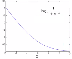
This plot shows the cost contribution of an example when y = 1 given z So if z is big, the cost is low. But if z is 0 or negative the cost contribution is high. This is why, when logistic regression sees a positive example, it tries to set \( \theta^T.x \) to be a very large term.
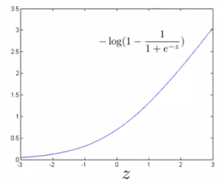
If y = 0 then only the second term matters. We can again plot it and get a similar graph. Here if z is small then the cost is low, But if s is large then the cost is massive
SVM cost functions from logistic regression cost functions
To build a SVM we must redefine our cost functions: When y = 1, Take the y = 1 function and create a new cost function. Instead of a curved line create two straight lines (magenta) which acts as an approximation to the logistic regression y = 1 function.
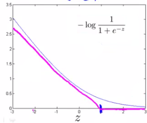
Take point (1) on the z axis, Flat from 1 onwards It Grows when we reach 1 or a lower number. This means we have two straight lines. Flat when cost is 0 Straight growing line after 1, So this is the new y=1 cost function. This gives the SVM a computational advantage and an easier optimization problem We call this function cost1(z).
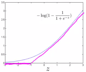
Similarly When y = 0 Do the equivalent with the y = 0 function plot. We call this function cost0(z). So here we define the two cost function terms for our SVM graphically.
The complete SVM cost function : As a comparison/reminder we have logistic regression below
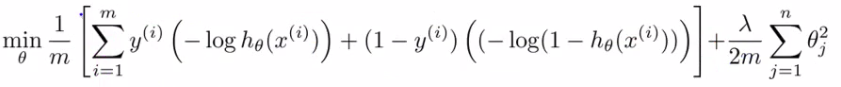
If this looks unfamiliar its because we previously had the - sign outside the expression. For the SVM we take our two logistic regression y = 1 and y = 0 terms described previously and replace with: \( \text{cost}_1(\theta^T.x), \text{cost}_2(\theta^T.x) \). So we get :
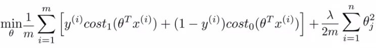
SVM notation is slightly different
In convention with SVM notation we rename a few things here:
Get rid of the 1/m terms. This is just a slightly different convention By removing 1/m we should get the same optimal values for 1/m is a constant, so should get same optimization. e.g. say you have a minimization problem which minimizes to x = 5 such as \( (x-5)^2 + 1 \). If your cost function * by a constant i.e. \( 10 [(x-5)^2 + 1] = 10(x-5)^2 + 10 \), you still generates the same minimal value.
For logistic regression we had two terms; Training data set term (i.e. that we sum over m) = A Regularization term (i.e. that we sum over n) = B So we could describe it as A + λB. Instead of parameterization this as A + λB For SVMs the convention is to use a different parameter called C So do CA + B If C were equal to 1/λ then the two functions (CA + B and A + λB) would give the same value
So, our overall equation is
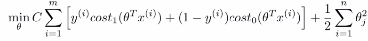
Unlike logistic, \( h_\theta(x) \) doesn't give us a probability, but instead we get a direct prediction of 1 or 0 So if \( \theta^T*x \) is equal to or greater than 0 --> \( h_\theta(x) \) = 1 Else --> \( h_\theta(x) \) = 0.