What are kernels and how do we use them? We have a training set and We want to find a non-linear boundary.

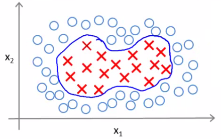
Come up with a complex set of polynomial features to fit the data Have \( h_\theta(x) \) which Returns 1 if the combined weighted sum of vectors (weighted by the parameter vector) is less than or equal to 0 or Else return 0.

Another way of writing this (new notation) is That a hypothesis computes a decision boundary by taking the sum of the parameter vector multiplied by a new feature vector f, which simply contains the various high order x terms

e.g. \( h_\theta(x) = θ_0+ θ_1f_1+ θ_2f_2 + θ_3f_3 \) Where \( f_1= x_1 \\ f_2 = x_1x_2 \\ f_3 = ... \)

i.e. not specific values, but each of the terms from your complex polynomial function Is there a better choice of feature f than the high order polynomials? As we saw with computer imaging, high order polynomials become computationally expensive

New features Define three features in this example (ignore x₀) Have a graph of x₁ vs. x₂ (don't plot the values, just define the space) Pick three points in that space

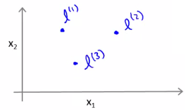
These points l₁, l₂, and l₃, were chosen manually and are called landmarks

Given x, define f₁ as the similarity between (x, l₁) = \( exp\frac{(- (|| x - l_1||^2 )} {2\sigma^2} \)

|| x - l₁ || is the euclidean distance between the point x and the landmark l₁ squared

If we remember our statistics, we know that σ is the standard deviation σ2 is commonly called the variance

So, f₂ is defined as f₂ = similarity(x, l₂) = exp(- (|| x - l₂ ||2 ) / 2σ2) And similarly f₃ = similarity(x, l₃) = exp(- (|| x - l₃ ||2 ) / 2σ2) This similarity function is called a kernel

This function is a Gaussian Kernel So, instead of writing similarity between x and l we might write f₁= k(x, l₁)

So lets see what these kernels do and why the functions defined make sense Say x is close to a landmark Then the squared distance will be ~0 So \( f_1 \sim exp(-\frac{0^2}{2\sigma^2})\)

Which is basically \( e^{-0} \) which is close to 1. Say x is far from a landmark, then the squared distance is big, which is gives e^{- large number} which gives a result that is close to zero.

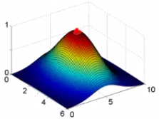
Each landmark defines a new feature. If we plot f₁ vs the kernel function we get a plot like this Notice that when x = [3,5] then f₁ = 1 As x moves away from [3,5] then the feature takes on values close to zero So this measures how close x is to this landmark.

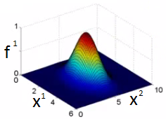
What does σ do? σ² is a parameter of the Gaussian kernel Defines the steepness of the rise around the landmark Above example σ² = 1 Below σ² = 0.5

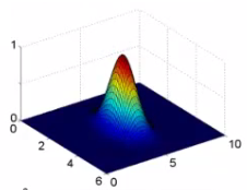
We see here that as you move away from x = [3,5] the feature f₁ falls to zero much more rapidly. The inverse can be seen if σ² = 3.

Given this definition, what kinds of hypotheses can we learn? With training examples x we predict "1" when \( θ_0 + θ_1f_1 + θ_2f_2 + θ_3f_3 >= 0 \)

For our example, lets say we've already run an algorithm and got the θ₀ = -0.5 θ₁ = 1 θ₂ = 1 θ₃ = 0

Given our placement of three examples, what happens if we evaluate an example at the magenta dot below?

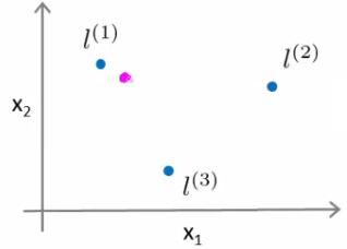
Looking at our formula, we know f₁ will be close to 1, but f₂ and f₃ will be close to 0

So if we look at the formula we have \( θ_0+ θ_1f_1 + θ_2f_2 + θ_3f_3 >= 0 \\ -0.5 + 1 + 0 + 0 = 0.5 \) 0.5 is greater than 1

If we had another point far away from all three

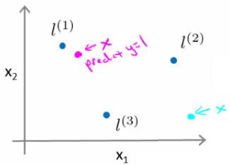
This equates to -0.5 So we predict 0 Considering our parameter, for points near l1 and l2 you predict 1, but for points near l3 you predict 0 Which means we create a non-linear decision boundary that goes a lil' something like this;

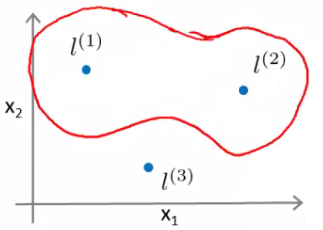
Inside we predict y = 1 Outside we predict y = 0 So this show how we can create a non-linear boundary with landmarks and the kernel function in the support vector machine

But How do we get/chose the landmarks What other kernels can we use (other than the Gaussian kernel)

Now, Where do we get the landmarks from? For complex problems we probably want lots of them.

Algorithm : Choosing the landmarks

Predict y = 1 if (θ^T f) >= 0

Because θ = [m+1 x 1] -- dimensions of the matrix ; And f = [m +1 x 1] -- dimensions of the matrix. We can multiply these.

So, this is how you make a prediction assuming you already have θ How do you get θ? . Given in the next section.

Use the SVM learning algorithm: Cost function given below

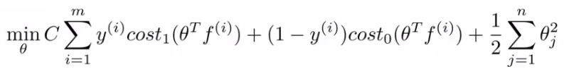
Now, we minimize using f as the feature vector instead of x. By solving this minimization problem you get the parameters for your SVM. In this setup, m = n because number of features is the number of training data examples we have

SVM parameters (C) : Bias and variance trade off is controlled by parameter 'C'. Must chose C carefully. C plays a role similar to 1/LAMBDA (where LAMBDA is the regularization parameter). Large C gives a hypothesis of low bias high variance --> overfitting Small C gives a hypothesis of high bias low variance --> underfitting

SVM parameters (σ2) Parameter for calculating f values Large σ2 - f features vary more smoothly - higher bias, lower variance Small σ2 - f features vary abruptly - low bias, high variance

Use SVM software packages (e.g. liblinear, libsvm) to solve parameters θ Need to specify Choice of parameter C Choice of kernel Choosing a kernel

We've looked at the Gaussian kernel Need to define σ (σ2)

When would you chose a Gaussian? If n is small and/or m is large e.g. 2D training set that's large

If you're using a Gaussian kernel then you may need to implement the kernel function e.g. a function fi = kernel(x1,x2) Returns a real number

Some SVM packages will expect you to define kernel Although, some SVM implementations include the Gaussian and a few others Gaussian is probably most popular kernel

NB - make sure you perform feature scaling before using a Gaussian kernel If you don't features with a large value will dominate the f value

Could use no kernel - linear kernel Predict y = 1 if (θT x) >= 0 So no f vector

Get a standard linear classifier Why do this? If n is large and m is small then Lots of features, few examples Not enough data - risk overfitting in a high dimensional feature-space

Other choice of kernel : Linear and Gaussian are most common. But few other choices exist.

Polynomial Kernel We measure the similarity of x and l by doing one of

\( (x^T . l)^2 \\ (x^T . l)^3 \\ (x^T . l+1)^3 \\ ... \\ (x^T . l+Const)^D \)

If they're similar then the inner product tends to be large Not used that often , hence Two parameters : Degree of polynomial (D) ; Number you add to l (Const)

Many packages have built in multi-class classification packages Otherwise use one-vs all method Not a big issue

Logistic regression vs. SVM When should you use SVM and when is logistic regression more applicable If n (features) is large vs. m (training set) e.g. text classification problem

Feature vector dimension is 10,000 Training set is 10 - 1000 Then use logistic regression or SVM with a linear kernel

If n is small and m is intermediate n = 1 - 1000 m = 10 - 10 000 Gaussian kernel is good

If n is small and m is large n = 1 - 1000 m = 50 000+ SVM will be slow to run with Gaussian kernel

In that case Manually create or add more features Use logistic regression or SVM with a linear kernel

Logistic regression and SVM with a linear kernel are pretty similar Do similar things Get similar performance

A lot of SVM's power is using diferent kernels to learn complex non-linear functions

For all these regimes a well designed Neural Network should work But, for some of these problems a NN might be slower - SVM well implemented would be faster

SVM has a convex optimization problem - so you get a global minimum

Files included in this exercise can be downloaded here ⇒ : Exercise-6