Anomaly Detection
Anomaly detection is a reasonably commonly used type of machine learning application. It can be thought of as a solution to an unsupervised learning problem. But, has aspects of supervised learning.
What is anomaly detection? Imagine you're an aircraft engine manufacturer. As engines roll off your assembly line you're doing Quality Assurance.
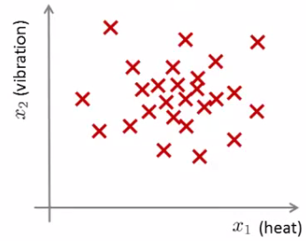
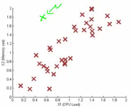
You measure some features from engines (e.g. heat generated and vibration) and the aim is to detect which engines are faulty. After the data collection, You now have a dataset X of x1 to xm (i.e. m engines were tested). Say we plot that dataset.
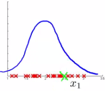
Next day you have a new engine. An anomaly detection method is used to see if the new engine is anomalous (when compared to the previous engines). If the new engine looks like this; (green cross in the plot given below)
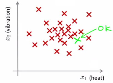
It must be Probably OK - as it looks like the ones we've seen before. But if the engine looks like this (green cross in the plot given below)
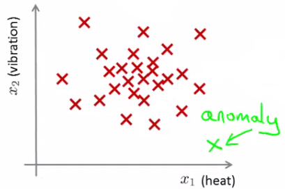
Then this looks like an anomalous data-point. More formally, We have a dataset which contains normal (data). Using that dataset as a reference point we can see if other examples are anomalous.
Anomaly Detection - Understanding
How do we do Anomaly Detection ? First, using our training dataset we build a model. We can assess this model using p(x). p(x) asks, "What is the probability that example x is normal".
Having built a model, if p(xtest) < ε --> flag this data point as an anomaly. If p(xtest) >= ε --> this is OK. ε is some threshold probability value which we define, depending on how sure we need/want to be.
We expect our model to (graphically) look something like this;
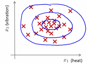
i.e. this would be our model if we had 2D data
Anomaly Detection - Applications
In Fraud detection, Users have activity associated with them, such as Length on time on-line, Location of login, Spending frequency etc.
Using this data we can build a model of what normal users' activity is like What is the probability of "normal" behavior?
Then we can Identify unusual users by sending their data through the model. Flag up anything that looks a bit weird and automatically block cards/transactions.
Manufacturing : Monitoring computers in data center. If you have many machines in a cluster then Computer features of machine are x1 = memory use, x2 = number of disk accesses/sec, x3 = CPU load.
In addition to the measurable features you can also define your own complex features such as x4 = CPU load/network traffic.
If you see an anomalous machine then it Maybe about to fail and you should Look at replacing bits from it.
The Gaussian distribution
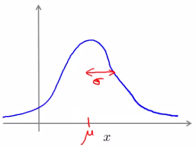
It is also called the normal distribution. Example Say x (data set) is made up of real numbers with Mean is μ and Variance is σ2. Then σ is also called the standard deviation - specifies the width of the Gaussian probability.
The data has a Gaussian distribution. Then we can write this ~ N(μ,σ2 ). ~ means = is distributed as. N -> means normal distribution, μ, σ2 represent the mean and variance, respectively. These are the two parameters of a Gaussian.
The distribution look as the figure below:
Gaussian equation is P(x : μ , σ2) (probability of x, parameterized by the mean and squared variance)
\( \frac{1}{\sqrt{2*\pi*\sigma}} exp(- \frac{(x - \mu)^2}{2\sigma^2}) \)
This specifies the probability of x taking a value
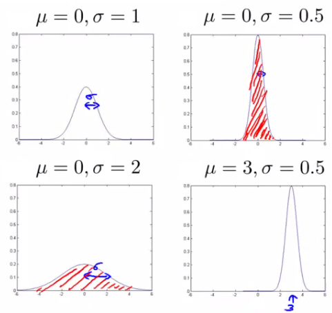
Some examples of Gaussians are given below: Note that Area is always the same, But width changes as standard deviation changes.
Parameter estimation problem
What is Parameter estimation problem? Say we have a data set of m examples.. Give each example is a real number - we can plot the data on the x axis as shown below.
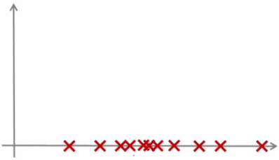
Problem is - say you suspect these examples come from a Gaussian distribution. Given the dataset can you estimate the distribution? Could be something like given in the below figure.
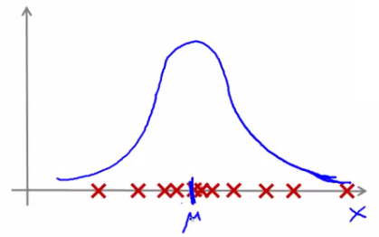
Seems like a reasonable fit - data seems like a higher probability of being in the central region, lower probability of being further away. Estimating μ and σ2. μ = average of examples and σ2 = standard deviation squared.
\( \sigma^2 = \frac{1}{m} \sum_{i = 1}^{m} (x^{(i)} - \mu)^2 \)
As a side comment : These parameters estimations are found using a technique known as the maximum likelihood estimation values for μ and σ2.
You can also replace 1/(m) or 1/(m-1) (as some of the books may have the other formula) doesn't make too much difference. Slightly different mathematical problems, but in practice it makes little difference.
Anomaly Detection - Algorithm
Steps :
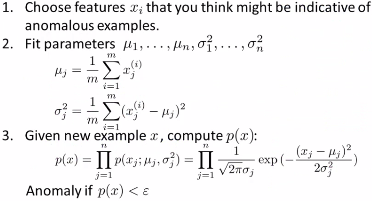
Chose features : Try to come up with features which might help identify something anomalous - may be unusually large or small values. More generally, chose features which describe the general properties. This is nothing unique to anomaly detection - it's just the idea of building a sensible feature vector
Fit parameters : Determine parameters for each of your examples μi and σi2. Fit is a bit misleading, really should just be "Calculate parameters for 1 to n". So you're calculating standard deviation and mean for each feature . You should of course used some vectorized implementation rather than a loop probably
compute p(x) : You compute the formula shown (i.e. the formula for the Gaussian probability). If the number is very small, very low chance of it being "normal"
Anomaly detection example
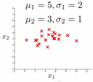
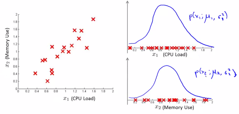
x1 : Mean is about 5, Standard deviation looks to be about 2.
x2 : Mean is about 3, Standard deviation about 1.
So we have the following system
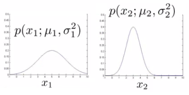
If we plot the Gaussian for x1 and x2 we get something like this
If you plot the product of these things you get a surface plot like this
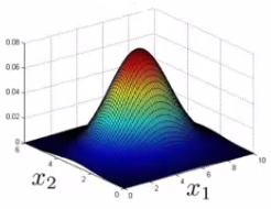
With this surface plot, the height of the surface is the probability - p(x). We can't always do surface plots, but for this example it's quite a nice way to show the probability of a 2D feature vector.
Check if a value is anomalous. Set epsilon as some value. Say we have two new data points new data-point has the values : x1test, x2test.
We compute p(x1test) = 0.436 >= epsilon (~40% chance it's normal) , so result is Normal. Then we compute p(x2test) = 0.0021 < epsilon (~0.2% chance it's normal). Hence it is Anomalous.
What this is saying is if you look at the surface plot, all values above a certain height are normal, all the values below that threshold are probably anomalous
Developing and evaluating and anomaly detection system
Previously we spoke about the importance of real-number evaluation of learning techniques. Often we need to make a lot of choices (e.g. features to use).
Hence, it is easier to evaluate your algorithm if it returns a single number to show if changes you made improved or worsened an algorithm's performance.
To develop an anomaly detection system quickly, would be helpful to have a way to evaluate your algorithm. Assume we have some labeled data. So far we've been treating anomalous detection with unlabeled data.
If you have labeled data it allows evaluation i.e. if you think something is anomalous you can be sure if it is or not.
So, taking our engine example. You have some labeled data : Data for engines which were non-anomalous -> y = 0 Data for engines which were anomalous -> y = 1.
Training set is the collection of normal examples. It is OK even if we have a few anomalous data examples. Next define Cross validation set and Test set.
For both assume you can include a few examples which have anomalous examples.
Example: Engines - Have 10 000 good engines and it is OK even if a few bad ones are there amongst the good ones. Thus we will have LOTS of y = 0 and about 20 flawed engines. Typically when y = 1 have 2-50 is normal and does not affect performance.
Split into Training set: 6000 good engines (y = 0), CV set: 2000 good engines, 10 anomalous and Test set: 2000 good engines, 10 anomalous. Ratio is 3:1:1.
Sometimes we see a different way of splitting. Take 6000 good in training, Same CV and test set (4000 good in each) different 10 anomalous, Or even 20 anomalous (same ones).
This is bad practice - should use different data in CV and test set.
Algorithm evaluation is performed as follows : Take trainings set { x1, x2, ..., xm }. Fit model p(x) On cross validation and test set, test the example x and assign y = 1 if p(x) < epsilon (anomalous) OR y = 0 if p(x) >= epsilon (normal).
Think of algorithm as trying to predict if something is anomalous. But you have a label so can check! Makes it look like a supervised learning algorithm.
What's a good metric to use for evaluation. As y = 0 is very common So classification error would be bad method for checking accuracy.
Compute fraction of true positives/false positive/false negative/true negative. Compute precision/recall. Compute F1-score.
If you have CV set you can see how varying epsilon effects various evaluation metrics. Then pick the value of epsilon which maximizes the score on your CV set. Evaluate algorithm using cross validation. Do final algorithm evaluation on the test set.
Anomaly detection vs. supervised learning
If we have labeled data, we not use a supervised learning algorithm? Here we'll try and understand when you should use supervised learning and when anomaly detection would be better.
Anomaly detection : Very small number of positive examples exists i.e. anamolous data points. Save positive examples just for CV and test set, hence for training set not enough examples are available.
Consider using an anomaly detection algorithm - Not enough data to "learn" positive examples. Have a very large number of negative examples. Use these negative examples for p(x) fitting. Only need negative examples for this.
Many "types" of anomalies. Hard for an algorithm to learn from positive examples when anomalies may look nothing like one another. So anomaly detection doesn't know what they look like, but knows what they don't look like.
In other words, it is easier for an algorithm to learn from data what is normal behavior as large examples of normal behaviour exist. But as very few examples of anamolous behavior exist we cannot have supervised learning to train algorithms for them.
Improving performance of an anamoly detector - Choosing features to use
One of the things which has a huge effect is which features are used. Non-Gaussian features : Plot a histogram of data to check it has a Gaussian. Often still works if data is non-Gaussian. Use hist command to plot histogram. Non-Gaussian data might look like this.
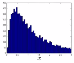
Can play with different transformations of the data to make it look more Gaussian Might take a log transformation of the data i.e. if you have some feature x1, replace it with log(x1)
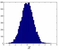
This looks much more Gaussian Or do log(x1+c) Play with c to make it look as Gaussian as possible Or do x1/2 Or do x1/3
Error analysis for anomaly detection : Good way of coming up with features. Like supervised learning error analysis procedure. Run algorithm on CV set. See which one it got wrong. Develop new features based on trying to understand why the algorithm got those examples wrong.
Example - data center monitoring Features in the dataset were x1 = memory use x2 = number of disk access/sec x3 = CPU load x4 = network traffic.
We suspect CPU load and network traffic grow linearly with one another. If server is serving many users, CPU is high and network is high. Fail case is infinite loop, so CPU load grows but network traffic is low. New feature is needed to detect this anamoly and we create it as - CPU load/network traffic.
Multivariate Gaussian distribution
This Is a slightly different technique which can sometimes catch some anomalies which non-multivariate Gaussian distribution anomaly detection fails to.
Unlabeled data set looks like this.
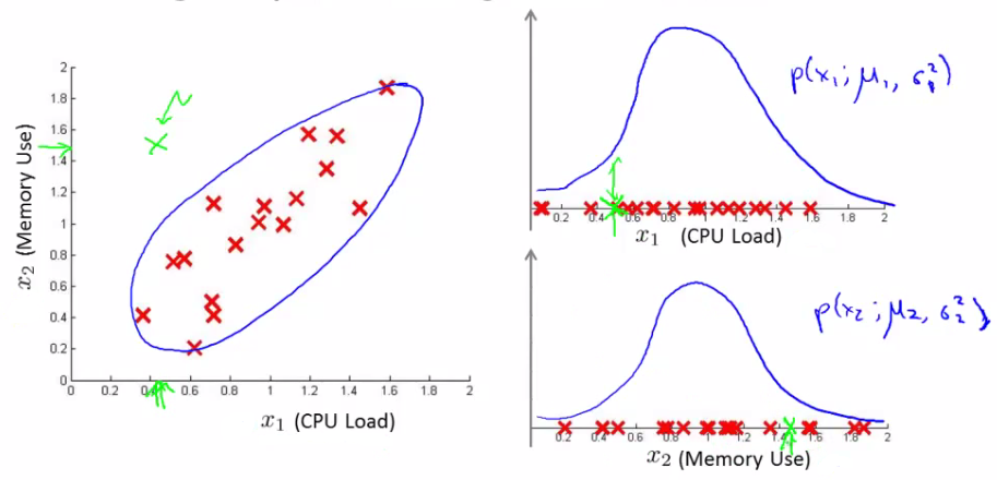
Say you can fit a Gaussian distribution to CPU load and memory use. Lets say in the test set we have an example which looks like an anomaly (e.g. x1 = 0.4, x2 = 1.5). Looks like most of data lies in a region far away from this example.
Here memory use is high and CPU load is low (if we plot x1 vs. x2 our green example looks miles away from the others). Problem is, if we look at each feature individually they may fall within acceptable limits - the issue is we know we shouldn't don't get those kinds of values together. But individually, they're both acceptable.
This is because our function makes probability prediction in concentric circles around the the means of both.
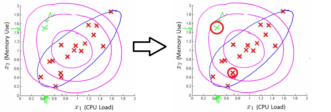
Probability of the two red circled examples is basically the same, even though we can clearly see the green one as an outlier.
Multivariate Gaussian distribution model
To get around this we develop the multivariate Gaussian distribution. Model p(x) all in one go, instead of each feature separately.
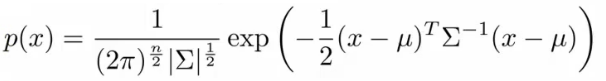
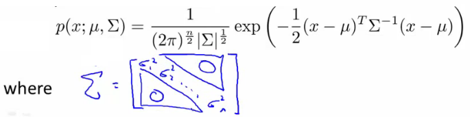
What are the parameters for this new model? μ - which is an n dimensional vector (where n is number of features). Σ - which is an [n x n] matrix - the covariance matrix. For the sake of completeness, the formula for the multivariate Gaussian distribution is as follows.
\( p(x; \mu , \Sigma) = \frac{1}{(2\pi)^{n/2}|\Sigma|^{1/2}} exp(- \frac{1}{2} (x - \mu)^T \Sigma^{-1} (x - \mu))\)
What does this mean? |Σ| = absolute value of Σ (determinant of sigma) This is a mathematic function of a matrix You can compute it in MATLAB using det(sigma).
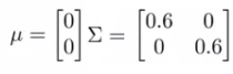
More importantly, what does this p(x) look like? 2D example
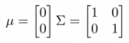
Sigma is sometimes call the identity matrix
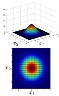
p(x) looks like this. For inputs of x1 and x2 the height of the surface gives the value of p(x). What happens if we change Sigma?
So now we change the plot to
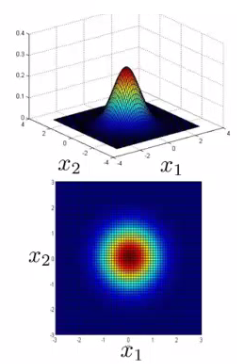
Now the width of the bump decreases and the height increases If we set sigma to be different values this changes the identity matrix and we change the shape of our graph
Using these values we can, therefore, define the shape of this to better fit the data, rather than assuming symmetry in every dimension
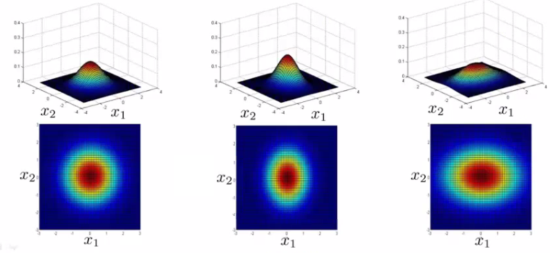
One of the cool things is you can use it to model correlation between data If you start to change the off-diagonal values in the covariance matrix you can control how well the various dimensions correlation
So we see here the final example gives a very tall thin distribution, shows a strong positive correlation
We can also make the off-diagonal values negative to show a negative correlation Hopefully this shows an example of the kinds of distribution you can get by varying sigma We can, of course, also move the mean (μ) which varies the peak of the distribution
Applying multivariate Gaussian distribution to anomaly detection
Saw some examples of the kinds of distributions you can model
Now let's take those ideas and look at applying them to different anomaly detection algorithms
As mentioned, multivariate Gaussian modeling uses the following equation; \( p(x; \mu , \Sigma) = \frac{1}{(2\pi)^{n/2}|\Sigma|^{1/2}} exp(- \frac{1}{2} (x - \mu)^T \Sigma^{-1} (x - \mu))\)
Which comes with the parameters μ and Σ Where μ - the mean (n-dimenisonal vector) Σ - covariance matrix ([nxn] matrix)
Parameter fitting/estimation problem If you have a set of examples {x1, x2, ..., xm }
The formula for estimating the parameters is \( \mu = \frac{1}{m} \sum_{i = 1}^{m} x^{(i)} \\ \Sigma = \frac{1}{m} \sum_{i = 1}^{m} (x^{(i)} - \mu)(x^{(i)} - \mu)^T \)
Using these two formulas you get the parameters
Anomaly detection algorithm with multivariate Gaussian distribution
Fit model - take data set and calculate μ and Σ using the formula above.
We're next given a new example (xtest) - see below
For it compute p(x) using the following formula for multivariate distribution.
Compare the value with ε (threshold probability value) if p(xtest) < ε --> flag this as an anomaly if p(xtest) >= ε --> this is OK
If you fit a multivariate Gaussian model to our data we build something like this
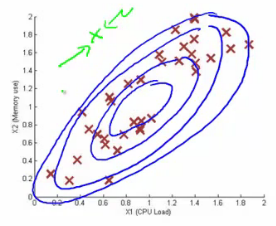
Which means it's likely to identify the green value as anomalous Finally, we should mention how multivariate Gaussian relates to our original simple Gaussian model (where each feature is looked at individually)
Original model corresponds to multivariate Gaussian where the Gaussians' contours are axis aligned i.e. the normal Gaussian model is a special case of multivariate Gaussian distribution
This can be shown mathematically Has this constraint that the covariance matrix sigma as ZEROs on the non-diagonal values
If you plug your variance values into the covariance matrix the models are actually identical
Original model vs. Multivariate Gaussian
| Original model | Multivariate Gaussian |
|---|---|
| Probably used more often | Used less frequently |
| There is a need to manually create features to capture anomalies where x1 and x2 take unusual combinations of values | Can capture feature correlation So no need to create extra values |
| So need to make extra features Might not be obvious what they should be | Less computationally efficient Must compute inverse of matrix which is [n x n] So lots of features is bad - makes this calculation very expensive So if n = 100 000 not very good |
| Much cheaper computationally Scales much better to very large feature vectors Even if n = 100 000 the original model works fine Works well even with a small training set e.g. 50, 100 | Needs for m > n i.e. number of examples must be greater than number of features If this is not true then we have a singular matrix (non-invertible) So should be used only in m >> n |
| Because of these factors it's used more often because it really represents a optimized but axis-symmetric specialization of the general model | If you find the matrix is non-invertible, could be for one of two main reasons m < n So use original simple model Redundant features (i.e. linearly dependent) i.e. two features that are the same If this is the case you could use PCA or sanity check your data |
Programming exercises : Anomaly Detection and Recommender Systems
Files included in this exercise can be downloaded here ⇒ : Exercise-8