• So far we have visualized relationships between two quantitative variables using scatterplots, and described the overall pattern of a relationship by considering its direction, form, and strength. We noted that assessing the strength of a relationship just by looking at the scatterplot is quite difficult, and therefore we need to supplement the scatterplot with some kind of numerical measure that will help us assess the strength.




• In this part, we will restrict our attention to the special case of relationships that have a linear form, since they are quite common and relatively simple to detect. More importantly, there exists a numerical measure that assesses the strength of the linear relationship between two quantitative variables with which we can supplement the scatterplot. We will introduce this numerical measure here and discuss it in detail.




• Even though from this point on we are going to focus only on linear relationships, it is important to remember that not every relationship between two quantitative variables has a linear form. We have actually seen several examples of relationships that are not linear. The statistical tools that will be introduced here are appropriate only for examining linear relationships, and as we will see, when they are used in nonlinear situations, these tools can lead to errors in reasoning.





• We can see that in both cases, the direction of the relationship is positive and the form of the relationship is linear. What about the strength? Recall that the strength of a relationship is the extent to which the data follow its form.




• The Correlation Coefficient—r The numerical measure that assesses the strength of a linear relationship is called the correlation coefficient, and is denoted by r. The correlation coefficient (r) is a numerical measure that measures the strength and direction of a linear relationship between two quantitative variables.




• r = \( \frac{1}{n-1} \sum_{i=1}^n \frac{x_i - \overline{x}}{S_x} \frac{y_i - \overline{y}}{S_y} \)




• The value of r ranges only from negative one to one. There is no way in which r can take values outside this range.




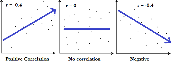
• The sign of r, either positive or negative, indicates the direction of the relationship. As expected, negative values of r indicate a negative relationship and positive values of r indicate a positive relationship.




• More importantly, r indicates the strength of the linear relationship. Values of r that are close to zero, either positive or negative, indicate a weak linear relationship.




• The closer r is to zero, the weaker the relationship. The extreme case of r equals zero indicates no linear relationship. Values of r close to negative one and one indicate that the linear relationship is strong.




• Values of r close to negative one indicate a strong negative linear relationship and the closer r is to negative one, the stronger their relationship.




• Values of r close to positive one indicate a strong positive linear relationship, and the closer r is to positive one, the stronger the relationship





• The correlation coefficient can only be interpreted as the measure of the strength of a linear relationship, so we need the scatterplot to verify that the relationship indeed looks linear.

Sample question: Find the value of the correlation coefficient r = \( \frac{n(\sum xy) - (\sum x)(\sum y)}{\sqrt{[n \sum x^2 - (\sum x)^2][n\sum y^2 - (\sum y)^2]}} \)from the following table:

Subject	Age x	Glucose Level y
1	43	99
2	21	65
3	25	79
4	42	75
5	57	87
6	59	81

Step 1:Make a chart. Use the given data, and add three more columns: xy, x², and y².

Subject	Age x	Glucose Level y	xy	x2	y2
1	43	99
2	21	65
3	25	79
4	42	75
5	57	87
6	59	81

Step 2: Multiply x and y together to fill the xy column. For example, row 1 would be 43 × 99 = 4,257.

Subject	Age x	Glucose Level y	xy	x2	y2
1	43	99	4257
2	21	65	1365
3	25	79	1975
4	42	75	3150
5	57	87	4959
6	59	81	4779

Step 3: Take the square of the numbers in the x column, and put the result in the x² column.

Subject	Age x	Glucose Level y	xy	x2	y2
1	43	99	4257	1849
2	21	65	1365	441
3	25	79	1975	625
4	42	75	3150	1764
5	57	87	4959	3249
6	59	81	4779	3481

Step 4: Take the square of the numbers in the y column, and put the result in the y² column.

Subject	Age x	Glucose Level y	xy	x2	y2
1	43	99	4257	1849	9801
2	21	65	1365	441	4225
3	25	79	1975	625	6241
4	42	75	3150	1764	5625
5	57	87	4959	3249	7569
6	59	81	4779	3481	6561

Step 5: Add up all of the numbers in the columns and put the result at the bottom of the column. The Greek letter sigma (Σ) is a short way of saying “sum of.”

Subject	Age x	Glucose Level y	xy	x2	y2
1	43	99	4257	1849	9801
2	21	65	1365	441	4225
3	25	79	1975	625	6241
4	42	75	3150	1764	5625
5	57	87	4959	3249	7569
6	59	81	4779	3481	6561
Σ	247	486	20485	11409	40022

From our table:

• Σx = 247
• Σy = 486
• Σxy = 20,485
• Σx² = 11,409
• Σy² = 40,022
• n is the sample size, in our case = 6

The correlation coefficient =

• 6(20,485) – (247 × 486) / [√[[6(11,409) – (247²)] × [6(40,022) – 486²]]]

= 0.5298

The range of the correlation coefficient is from -1 to 1. Our result is 0.5298 or 52.98%, which means the variables have a moderate positive correlation.

• The correlation does not change when the units of measurement of either one of the variables change. In other words, if we change the units of measurement of the explanatory variable and/or the response variable, the change has no effect on the correlation (r).




• The same is true for changing the units of the explanatory variable, or of both variables. Thus, correlation (r) is unitless. It is just a number.





• The correlation measures only the strength of a linear relationship between two variables. It ignores any other type of relationship, no matter how strong it is. For example, consider the relationship between the average fuel usage of driving a fixed distance in a car, and the speed at which the car drives





• Our data describe a fairly simple curvilinear relationship: the amount of fuel consumed decreases rapidly to a minimum for a car driving 60 kilometers per hour, and then increases gradually for speeds exceeding 60 kilometers per hour. The relationship is very strong, as the observations seem to perfectly fit the curve.




• Although the relationship is strong, the correlation r = -0.172 indicates a weak linear relationship. This makes sense considering that the data fails to adhere closely to a linear form. The correlation is useless for assessing the strength of any type of relationship that is not linear (including relationships that are curvilinear, such as the one in our example)





• The correlation is useless for assessing the strength of any type of relationship that is not linear (including relationships that are curvilinear, such as the one in our example). Beware, then, of interpreting the fact that r is close to 0 as an indicator of a weak relationship rather than a weak linear relationship. This example also illustrates how important it is to always look at the data in the scatterplot because, as in our example, there might be a strong nonlinear relationship that r does not indicate.




• Since the correlation was nearly zero when the form of the relationship was not linear, we might ask if the correlation can be used to determine whether or not a relationship is linear.




• The correlation by itself is not sufficient to determine whether a relationship is linear. To see this, let's consider the study that examined the effect of monetary incentives on the return rate of questionnaires. Below is the scatterplot relating the percentage of participants who completed a survey to the monetary incentive that researchers promised to participants, in which we find a strong curvilinear relationship





• The relationship is curvilinear, yet the correlation r = 0.876 is quite close to 1.




• In the last two examples, we have seen two very strong curvilinear relationships, one with a correlation close to 0 and one with a correlation close to 1. Therefore, the correlation alone does not indicate whether a relationship is linear. The important principle here is:




• The correlation is heavily influenced by outliers. The way in which the outlier influences the correlation depends upon whether or not the outlier is consistent with the pattern of the linear relationship.

Previous

Next