• Purpose of Statistics Package Exercises : The Probability & Statistics course focuses on the processes you use to convert data into useful information. This involves




1. Collecting data,




2. Summarizing data, and




3. Interpreting data.




• In addition to being able to apply these processes, you can learn how to use statistical software packages to help manage, summarize, and interpret data. The statistics package exercises included throughout the course provide you the opportunity to explore a dataset and answer questions based on the output using R, Statcrunch, TI Calculator, Minitab, or Excel. In each exercise, you can choose to view instructions for completing the activity in R, Statcrunch, TI Calculator, Minitab, or Excel, depending on which statistics package you choose to use.




• The statistics package exercises are an extension of activities already embedded in the course and require you to use a statistics package to generate output and answer a different set of questions.




• To Download R




1. To download R, a free software environment for statistical computing and graphics, go to: https://www.r-project.org/ This link opens in a new tab and follow the instructions provided.




• Using R




1. Throughout the statistics package exercises, you will be given commands to execute in R. You can use the following steps to avoid having to type all of these commands in by hand:




2. Highlight the command with your mouse.




3. On the browser menu, click "Edit," then "Copy."




4. Click on the R command window, then at the top of the R window, click "Edit," then "Paste."




5. You may have to press to execute the command.




• R Version




1. The R instructions are current through version 3.2.5 released on April 14, 2016. Instructions in these statistics package exercises may not work with newer releases of R.




2. For help with installing R for MAC OS X or Windows click here

• The purpose of this activity is to discuss how in some cases exploratory data analysis can help you determine whether the conditions that allow us to use the z-test for the population mean (μ) are met.




• Background: In the Exploratory Data Analysis unit, we stressed that in general, it is always a good idea to look at your data (if the actual data are given). Moreover, related to our discussion now, looking at the data can be very helpful when trying to determine whether you can reliably use the test. In both of our leading examples, the data summaries (sample size, sample mean) were given rather than the raw data, but in practice, you are often working with the raw data. In example 1, we were told the SAT-M scores vary normally in the population, so even though the sample size (n = 4) was quite small, we could proceed with the test. In example 2, the sample size was large enough (n = 100) for us to proceed with the test even though we do not know whether the concentration level varies normally.




• Now imagine the following situation: A health educator at a small college wants to determine whether the exercise habits of male students in the college are similar to the exercise habits of male college students in general. The educator chooses a random sample of 20 male students and records the time they spend exercising in a typical week. Do the data provide evidence that the mean time male students in the college spend exercising in a typical week differs from the mean time for male college students in general (which is 8 hours)?




• Comment: Whether σ is known or not is really not relevant to this activity.




• 




• Here is a situation in which we do not have any information about whether the variable of interest, "time" (time spent exercising in a typical week) varies normally or not, and the sample size (n = 20) is not really large enough for us to be certain that the Central Limit Theorem applies. Recall from our discussion on the Central Limit Theorem that unless the distribution of "time" is extremely skewed and/or has extreme outliers, a sample of size 20 should be fine. However, how can we be sure that is, indeed, the case?




• If only the data summaries are given, there is really not a lot that can be done. You can say something like: "I'll proceed with the test assuming that the distribution of the variable "time" is not extremely skewed and does not have extreme outliers." If the actual data are given, you can make a more informed decision by looking at the data using a histogram. Even though the histogram of a sample of size 20 will not paint the exact picture of how the variable is distributed in the population, it could give a rough idea.




• R Instructions




1. To open R with the data set preloaded, right-click here and choose "Save Target As" to download the file to your computer. Then find the downloaded file and double-click it to open it in R.




2. The data have been loaded into the data frame time . Enter the command




1. 
   time




3. to see the data. There are 4 columns (named time1 through time4 ) representing 4 different samples of size 20 in the data frame.




4. To create a histogram of the column time1 with R, enter the command:




1. 
   hist(time$time1,xlab="Time Exercising Per Week", main="Sample 1")




5. Now change time1 to time2 , time3 , and time4 in the code above to see the histogram for each time column.




6. Note: You can modify the x-label and title as you choose.

View Answer

Comments:

• It is always a good idea to look at the data and get a sense of their pattern regardless of whether you actually need to do it in order to assess whether the conditions are met.




• This idea of looking at the data is not only relevant to the z-test, but to tests in general. In particular, we'll see that in the case where σ is unknown (which we'll discuss next) the conditions that allow us to safely use the test are the same as the conditions in this case, so the ideas of this activity directly apply to that case as well.




• Also, as you'll see, in the next module—inference for relationships—doing exploratory data analysis before inference will be an integral part of the process.

• The purpose of this activity is teach you to run the z-test for the population mean while exploring the effect of sample size on the significance of the results.




• Background:




• Recall example 1 that we've just completed:




• 




• Even though the sample mean was 550, which is substantially greater than the null value, 500, this result was not significant, since it was based on data obtained from only 4 students. In other words, the data did not provide enough evidence to reject Ho and conclude that the mean SAT-M score of all Ross College students is larger than 500, the national mean. If this sample mean were obtained from 5 students, would that result be significant? If not, would 6 be enough? In other words, what is the smallest sample size for which a sample of \( \overline{x} = 550 \) would be significant? In this activity, we will use statistical software to explore this question.




• Comment: If you think about it, this question is not very practical, because you do not know in advance what the sample mean will be, but it is intuitive enough that it will help you get a better sense of how the sample size affects the significance of the results.




• R Instructions




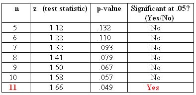
1. For n = 4, we know that the result x̄ = 550 is not significant. Using the R instructions below and starting with n = 5 (and going up), create and fill in a table where the column headings are "n," "z (test statistic)," "p-value," and "significant at the 0.05 level (yes/no)." Stop after the first time your result becomes significant at the 0.05 significance level.




2. We can use the following code to test the significance of the test under different sample size scenarios, n = 5 to n = 15.




3. Create a list of numbers 5,6,7,...,15 to represent various sample sizes:




1. n=5:15




4. Calculate the z-scores for each sample size:




1. z=(550-500)/(100/sqrt(n))




5. Calculate the p-values.




1. pvalue=1-pnorm(z)




6. Test whether the p-values are significant at 0.05. TRUE=Significant, FALSE=Not Significant:




1. significance=c(pvalue<0.05)




7. Compile the information into a table:




1. data.frame(n,z,pvalue,significance)

View Answer