Introduction to Statistics Package Exercises
Purpose of Statistics Package Exercises : The Probability & Statistics course focuses on the processes you use to convert data into useful information. This involves
Collecting data,
Summarizing data, and
Interpreting data.
In addition to being able to apply these processes, you can learn how to use statistical software packages to help manage, summarize, and interpret data. The statistics package exercises included throughout the course provide you the opportunity to explore a dataset and answer questions based on the output using R, Statcrunch, TI Calculator, Minitab, or Excel. In each exercise, you can choose to view instructions for completing the activity in R, Statcrunch, TI Calculator, Minitab, or Excel, depending on which statistics package you choose to use.
The statistics package exercises are an extension of activities already embedded in the course and require you to use a statistics package to generate output and answer a different set of questions.
To Download R
To download R, a free software environment for statistical computing and graphics, go to: https://www.r-project.org/ This link opens in a new tab and follow the instructions provided.
Using R
Throughout the statistics package exercises, you will be given commands to execute in R. You can use the following steps to avoid having to type all of these commands in by hand:
Highlight the command with your mouse.
On the browser menu, click "Edit," then "Copy."
Click on the R command window, then at the top of the R window, click "Edit," then "Paste."
You may have to press
to execute the command. R Version
The R instructions are current through version 3.2.5 released on April 14, 2016. Instructions in these statistics package exercises may not work with newer releases of R.
For help with installing R for MAC OS X or Windows click here
Statistics Package Exercise: Testing for a Linear Relationship
The purpose of this activity is to give you guided practice in testing whether the data provide evidence of a significant linear relationship, and in verifying that the basic conditions under which the results of such a test are reliable are met.
Recall the example from the previous activity:
A method for predicting IQ as soon as possible after birth could be important for early intervention in cases such as brain abnormalities or learning disabilities. It has been thought that greater infant vocalization (for instance, more crying) is associated with higher IQ. In 1964, a study was undertaken to see if IQ at 3 years of age is associated with amount of crying at newborn age. In the study, 38 newborns were made to cry after being tapped on the foot and the number of distinct cry vocalizations within 20 seconds was counted. The subjects were followed up at 3 years of age and their IQs were measured
R Instructions
To open R with the data set preloaded, right-click here and choose "Save Target As" to download the file to your computer. Then find the downloaded file and double-click it to open it in R.
The data have been loaded into the data frame baby . Enter the command
baby
to see the data. The two variables in the data frame are cry.count and IQ .
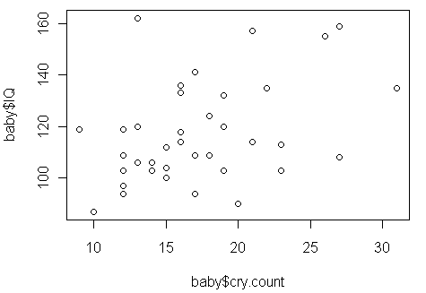
We would now like to test whether the observed (weak-to-moderate) linear relationship between cry count and IQ is significant (in other words, we would like to carry out the "t-test for the slope" for this example)
- Explanation :
The appropriate hypotheses (for the t-test for the slope) in this case are: Ho: There is no linear relationship between cry count and IQ. Ha: There is a significant linear relationship between cry count and IQ. What we are trying to assess using this test is whether there is evidence that the (weak-to-moderate) linear relationship that was observed between cry count and IQ in the sample we took also exists among infants in the general population.
- Explanation :
Let's start with the issue of independence: According to the paper, the 38 infants were a sample of infants born at the Long Island Jewish Hospital at the time of the study. Given this information, we can assume that the observations are independent (even though it doesn't explicitly say that the sample was random). The only obvious way that the independence assumption would be violated is if twins (or triplets ...) were included in the study, which we can assume was not the case. Comment: Even though the sample was chosen from a specific hospital (rather than from the "entire population of infants"), unless the infants who were born in this specific hospital at the time of the study were systematically different from infants in general in some relevant way, it will still be reasonable to attempt to generalize the results to infants in general. As for the other conditions: The relationship seems linear (even though it is moderately weak), the scatterplot does not display any alarming outliers, and the sample size is reasonably large (n = 38).
Statistics Package Exercise: Testing for a Linear Relationship
R Instructions
To carry out the test, enter the following command into R:
model=lm(baby$IQ~baby$cry.count)
summary(model)
The results include the following:
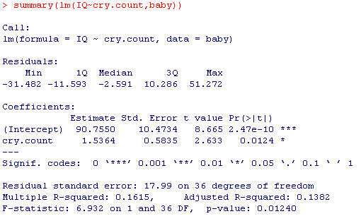
Estimates and standard errors of the intercept and slope t-Test statistic and p-value to test the two sided alternative β_1 ≠ 0 as well as a test for the intercept not equal to zero, which we generally ignore
The R^2 value (multiple R-squared), which is equivalent to the correlation squared, and measure of the proportion of variability in the response explained by the model The results of an equivalent test for the significance of the slope using an ANOVA approach
- Explanation :
The p-value of the test is 0.012. The small p-value (in particular, smaller than .05) tells us that it would be quite unlikely (1.2% chance) to get data like those observed just by chance. The data, therefore provide enough evidence for us to conclude that there is a significant linear relationship among infants between vocalization right after birth (as measured by cry count) and IQ at age 3.
Statistics Package Exercise: Making Predictions with a Least Squares Regression Line
The purpose of this activity is to complete our discussion about our example that examines the relationship between vocalization soon after birth and IQ at age three. So far we explored the data using a scatterplot supplemented with the correlation r:

and discovered that the data display a moderately weak positive linear relationship. In addition, when we carried out the t-test for assessing the significance of this linear relationship:

We concluded (based on the small p-value of 0.012) that the data provide fairly strong evidence of a moderately weak linear relationship between cry count soon after birth and IQ and age 3.
We would now like to consider using the least squares regression line for predicting IQ at age 3 based on cry count soon after birth. Plot the least squares regression line on the scatterplot:
R Instructions
To open R with the data set preloaded, right-click here and choose "Save Target As" to download the file to your computer. Then find the downloaded file and double-click it to open it in R.
The data have been loaded into the data frame baby . Enter the command
baby
to see the data. The two variables in the data frame are cry.count and IQ .
Let's rerun the previous code to acquire the plot and equation.
plot(baby$cry.count,baby$IQ, xlab="Number of Crying Events", ylab="IQ")
model=lm(baby$IQ~baby$cry.count)
abline(model)
cf=coef(model)
cf
legend(10,160,legend=paste("IQ = ", round(cf[1],1), "+", round(cf[2],2), "(cry.count)"))
- Explanation :
The least squares regression line is IQ = 90.8 + 1.54(cry count), and this graph displays it on the scatterplot: While the line captures the general linear trend of the data, it does not fit the data very well due to the moderately weak linearity in the data. Visually, we see that the data points do not lay close to the line, resulting in a relatively poor fit of the line to the data.
- Explanation :
The predicted IQ is obtained by plugging in a cry count of 25 into the regression line. We therefore obtain: Predicted IQ = 90.8 + 1.54 * 25 = 129.3. Here is the graph:. It should be noted, however, that due to the moderately weak linearity, this prediction is not very accurate in the sense that the actual IQ level can be either much lower or much higher than this predicted value (in the same way that many of the data points are well below or above the line). In fact, given how far the data points are from the line, the IQ could be roughly anywhere between 90 and 167 as this graph displays: Our prediction of the IQ being 129 is therefore not very accurate.