Introductory Video

• The Machine Learning course includes several programming assignments which you’ll need to finish to complete the course. The assignments require the Octave scientific computing language.




• Octave is a free, open-source application available for many platforms. It has a text interface and an experimental graphical one. Octave is distributed under the GNU Public License, which means that it is always free to download and distribute.




• Use Download to install Octave for windows. "Warning: Do not install Octave 4.0.0";




• Installing Octave on GNU/Linux : On Ubuntu, you can use: sudo apt-get update && sudo apt-get install octave. On Fedora, you can use: sudo yum install octave-forge

• Below commands can be copied and executed in the octave prompt one by one:




• Alternatively: Download octave script and run it in octave using command source("1.m"). Note : You may have to set octave to current working directory first.




• Comments are indicated in octave by putting % before the line




• %% elementary operations
  
  5+6 % ans =  11
  
  3-2 % ans =  1
  
  5*8 % ans =  40
  
  1/2 % ans =  0.50000
  
  2^6 % ans =  64
  
  1 == 2 % false - ans = 0
  
  1 ~= 2 % true. note, not "!=" ans = 1
  
  1 && 0 % ans = 0
  
  1 || 0 % ans = 1
  
  xor(1,0) % ans = 1
  
  %% variable assignment
  
  a = 3; % semicolon suppresses output
  
  b = 'hi';
  
  c = 3>=1;
  
  % Displaying them:
  
  a = pi
  
  disp(a)
  
  disp(sprintf('2 decimals: %0.2f', a)) % 2 decimals: 3.14
  
  disp(sprintf('6 decimals: %0.6f', a)) % 6 decimals: 3.141593
  
  format long a % a =  3.14159265358979
  
  format short a % a =  3.1416
  
  %% vectors and matrices
  
  A = [1 2; 3 4; 5 6]
  
  #{
  A =
  
     1   2
     3   4
     5   6
  #}
  
  v = [1 2 3]
  
  #{
  v =
  
     1   2   3
  #}
     
  v = [1; 2; 3]
  
  #{
  v =
  
     1
     2
     3
  #}
  
  v = 1:0.1:2 % from 1 to 2, with stepsize of 0.1. Useful for plot axes
  
  #{
  v =
  
   Columns 1 through 8:
  
      1.0000    1.1000    1.2000    1.3000    1.4000    1.5000    1.6000    1.7000
  
   Columns 9 through 11:
  
      1.8000    1.9000    2.0000
  #}
  
  v = 1:6 % from 1 to 6, assumes stepsize of 1 (row vector)
  
  #{
  v =
  
     1   2   3   4   5   6
  #}
  
  C = 2*ones(2,3) % same as C = [2 2 2; 2 2 2]
  
  #{
  C =
  
     2   2   2
     2   2   2
  #}
  
  w = ones(1,3) % 1x3 vector of ones
  
  #{
  w =
  
     1   1   1
  #}
  
  w = zeros(1,3)
  
  #{
  w =
  
     0   0   0
  #}
  
  w = rand(1,3) % drawn from a uniform distribution
  
  #{
  w =
  
     0.21612   0.37176   0.98264
  #}
  
  w = randn(1,3)% drawn from a normal distribution (mean=0, var=1)
  
  #{
  w =
  
     0.038128  -0.426170   0.114072
  #}
  
  w = -6 + sqrt(10)*(randn(1,10000)); % (mean = ‐6, var = 10) ‐ note: add the
  semicolon
  
  hist(w) % plot histogram using 10 bins (default)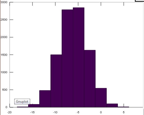
  
  
  
  hist(w,50) % plot histogram using 50 bins
  
  
  
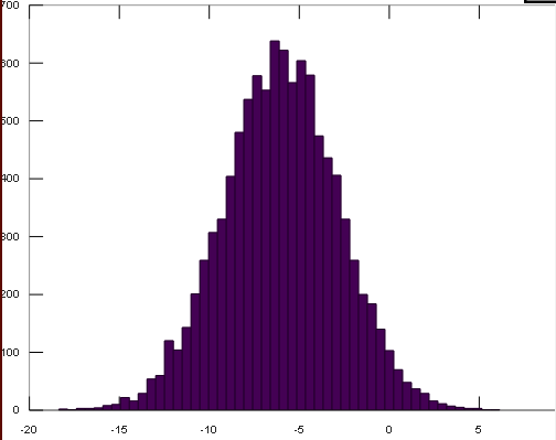  % note: if hist() crashes, try "graphics_toolkit('gnu_plot')"
  
  I = eye(4) % 4x4 identity matrix
  
  #{
  I =
  
  Diagonal Matrix
  
     1   0   0   0
     0   1   0   0
     0   0   1   0
     0   0   0   1
  #}
  
  % help function
  help eye
  help rand
  help help
  

• Below commands can be copied and executed in the octave prompt one by one:




• Comments are indicated in octave by putting % before the line




• 
  
  %% dimensions
  sz = size(A) % 1x2 matrix: [(number of rows) (number of columns)]
  size(A,1) % number of rows
  size(A,2) % number of cols
  length(v) % size of longest dimension
  A(3,2) % indexing is (row,col)
  A(2,:) % get the 2nd row.
  % ":" means every element along that dimension
  A(:,2) % get the 2nd col
  A([1 3],:) % print all the elements of rows 1 and 3
  A(:,2) = [10; 11; 12] % change second column
  A = [A, [100; 101; 102]]; % append column vec
  A(:) % Select all elements as a column vector.
  % Putting data together
  A = [1 2; 3 4; 5 6]
  B = [11 12; 13 14; 15 16] % same dims as A
  C = [A B] % concatenating A and B matrices side by side
  C = [A, B] % concatenating A and B matrices side by side
  C = [A; B] % Concatenating A and B top and bottom
  
  
  

• Below commands can be copied and executed in the octave prompt one by one:




• Comments are indicated in octave by putting % before the line




• 
  %% initialize variables
  A = [1 2;3 4;5 6]
  B = [11 12;13 14;15 16]
  C = [1 1;2 2]
  v = [1;2;3]
  %% matrix operations
  A * C % matrix multiplication
  A .* B % element‐wise multiplication
  % A .* C or A * B gives error ‐ wrong dimensions
  A .^ 2 % element‐wise square of each element in A
  1./v % element‐wise reciprocal
  log(v) % functions like this operate element‐wise on vecs or matrices
  exp(v)
  abs(v)
  -v % -1*v
  v + ones(length(v), 1)
  % v + 1 % same
  A' % matrix transpose
  %% misc useful functions
  % max (or min)
  a = [1 15 2 0.5]
  val = max(a)
  [val,ind] = max(a) % val ‐ maximum element of the vector a and index ‐ index
  value where maximum occur
  val = max(A) % if A is matrix, returns max from each column
  % compare values in a matrix & find
  a < 3 % checks which values in a are less than 3
  find(a < 3) % gives location of elements less than 3
  A = magic(3) % generates a magic matrix ‐ not much used in ML algorithms
  [r,c] = find(A>=7) % row, column indices for values matching comparison
  % sum, prod
  sum(a)
  prod(a)
  floor(a) % or ceil(a)
  max(rand(3),rand(3))
  max(A,[],1) %‐ maximum along columns(defaults to columns ‐ max(A,[]))
  max(A,[],2) %‐ maximum along rows
  A = magic(9)
  sum(A,1)
  sum(A,2)
  sum(sum( A .* eye(9) ))
  sum(sum( A .* flipud(eye(9)) ))
  % Matrix inverse (pseudo‐inverse)
  pinv(A) % inv(A'*A)*A'
  
  

• Below commands can be copied and executed in the octave prompt one by one:




• Comments are indicated in octave by putting % before the line




• %% plotting
  t = [0:0.01:0.98];
  y1 = sin(2*pi*4*t);
  plot(t,y1);
  y2 = cos(2*pi*4*t);
  hold on; % "hold off" to turn off
  plot(t,y2,'r');
  xlabel('time');
  ylabel('value');
  legend('sin','cos');
  title('my plot');
  print ‐dpng 'myPlot.png'
  close; % or, "close all" to close all figs
  figure(1); plot(t, y1);
  figure(2); plot(t, y2);
  figure(2), clf; % can specify the figure number
  subplot(1,2,1); % Divide plot into 1x2 grid, access 1st element
  plot(t,y1);
  subplot(1,2,2); % Divide plot into 1x2 grid, access 2nd element
  plot(t,y2);
  axis([0.5 1 ‐1 1]); % change axis scale
  %% display a matrix (or image)
  figure;
  imagesc(magic(15)), colorbar, colormap gray;
  % comma‐chaining function calls.
  a=1,b=2,c=3
  a=1;b=2;c=3;
  
  

• Below commands can be copied and executed in the octave prompt one by one:




• Comments are indicated in octave by putting % before the line




• v = zeros(10,1);
  for i=1:10,
  v(i) = 2^i;
  end;
  % Can also use "break" and "continue" inside for and while loops to control
  execution.
  i = 1;
  while i <= 5,
  v(i) = 100;
  i = i+1;
  end
  i = 1;
  while true,
  v(i) = 999;
  i = i+1;
  if i == 6,
  break;
  end;
  end
  if v(1)==1,
  disp('The value is one!');
  elseif v(1)==2,
  disp('The value is two!');
  else
  disp('The value is not one or two!');
  end
  
  

• Below commands can be copied and executed in the octave prompt one by one:




• Comments are indicated in octave by putting % before the line




• To create a function, type the function code in a text editor (e.g. gedit or notepad), and save the file as "functionName.m" so for below example file should be saved as "squareThisNumber.m" Example function:




• function y = squareThisNumber(x)
  y = x^2;
  




• To call the function in Octave, do either: 1) Navigate to the directory of the functionName.m (squareThisNumber.m) file and call the function




• % Navigate to directory:
  
  cd /path/to/function
  
  % Call the function:
  
  functionName(args)
  




• 2) Add the directory of the function to the load path and save it:You should not use addpath/savepath for any of the assignments in this course. Instead use 'cd' to change the current working directory.




• % To add the path for the current session of Octave:
  
  addpath('/path/to/function/')
  
  % To remember the path for future sessions of Octave, after executing
  
  addpath above, also do:
  savepath
  
  Octave's functions can return more than one value:
  




• function [y1, y2] = squareandCubeThisNo(x)
  y1 = x^2
  y2 = x^3
  




• [a,b] = squareandCubeThisNo(x)