Introductory Video

• The Machine Learning course includes several programming assignments which you’ll need to finish to complete the course. The assignments require the Octave scientific computing language.




• Octave is a free, open-source application available for many platforms. It has a text interface and an experimental graphical one. Octave is distributed under the GNU Public License, which means that it is always free to download and distribute.




• Use Download to install Octave for windows. "Warning: Do not install Octave 4.0.0";




• Installing Octave on GNU/Linux : On Ubuntu, you can use: sudo apt-get update && sudo apt-get install octave. On Fedora, you can use: sudo yum install octave-forge

• In this exercise, you will implement linear regression and get to see it work on data. Before starting on this programming exercise, we strongly recommend completing the previous chapters.




• To get started with the exercise, you will need to download the Download and unzip its contents to the directory where you wish to complete the exercise.




• If needed, use the cd command in Octave/MATLAB to change to this directory before starting this exercise.




• You can also find instructions for installing Octave/MATLAB in the “Environment Setup Instructions” of the course website.

• ex1.m - Octave/MATLAB script that steps you through the exercise




• ex1 multi.m - Octave/MATLAB script for the later parts of the exercise




• ex1data1.txt - Dataset for linear regression with one variable




• ex1data2.txt - Dataset for linear regression with multiple variables




• warmUpExercise.m - Simple example function in Octave/MATLAB




• plotData.m - Function to display the dataset




• computeCost.m - Function to compute the cost of linear regression




• gradientDescent.m - Function to run gradient descent




• Throughout the exercise, you will be using the script ex1.m. This script set up the dataset for the problems and make calls to functions that you will write. You do not need to modify either of them. You are only required to modify functions in other files, by following the instructions in this assignment.




• For this programming exercise, you are only required to complete the first part of the exercise to implement linear regression with one variable.

• The first part of ex1.m gives you practice with Octave/MATLAB syntax and the homework submission process. In the file warmUpExercise.m, you will find the outline of an Octave/MATLAB function. Modify it to return a 5 x 5 identity matrix by filling in the following code:




• A = eye(5);




• When you are finished, run ex1.m (assuming you are in the correct directory, type “ex1” at the Octave/MATLAB prompt) and you should see output similar to the following:




• ans =
  Diagonal Matrix
  1 0 0 0 0
  0 1 0 0 0
  0 0 1 0 0
  0 0 0 1 0
  0 0 0 0 1
  




• Now ex1.m will pause until you press any key, and then will run the code for the next part of the assignment. If you wish to quit, typing ctrl-c will stop the program in the middle of its run.

• In this part of this exercise, you will implement linear regression with one variable to predict profits for a food truck. Suppose you are the CEO of a restaurant franchise and are considering different cities for opening a new outlet. The chain already has trucks in various cities and you have data for profits and populations from the cities.




• You would like to use this data to help you select which city to expand to next.




• The file ex1data1.txt contains the dataset for our linear regression problem. The first column is the population of a city and the second column is the profit of a food truck in that city. A negative value for profit indicates a loss.




• The ex1.m script has already been set up to load this data for you.

Three Steps of this exercise

• Complete plotData.m




• Complete computeCost.m




• Complete gradientDescent.m




• Note : For each step its introduction , a small tutorial and test cases to check implementation are given.

• Before starting on any task, it is often useful to understand the data by visualizing it. For this dataset, you can use a scatter plot to visualize the data, since it has only two properties to plot (profit and population). (Many other problems that you will encounter in real life are multi-dimensional and can’t be plotted on a 2-d plot.)




• In ex1.m, the dataset is loaded from the data file into the variables X and y:




• 
  data = load('ex1data1.txt'); % read comma separated data
  X = data(:, 1); y = data(:, 2);
  m = length(y); % number of training examples
  




• Next, the script calls the plotData function to create a scatter plot of the data. Your job is to complete plotData.m to draw the plot; modify the file and fill in the following code:




• 
  plot(x, y, 'rx', 'MarkerSize', 10); % Plot the data
  ylabel('Profit in $10,000s'); % Set the y−axis label
  xlabel('Population of City in 10,000s'); % Set the x−axis label
  




• Now, when you continue to run ex1.m, our end result should look like Figure 1, with the same red “x” markers and axis labels. To learn more about the plot command, you can type help plot at the Octave/MATLAB command prompt or to search online for plotting documentation.




• (To change the markers to red “x”, we used the option ‘rx’ together with the plot command, i.e., plot(..,[your options here],.., ‘rx’); )

1. In ex1.m, we have already set up the data for linear regression. In the following lines, we add another dimension to our data to accommodate the θ0 intercept term. We also initialize the initial parameters to 0 and the learning rate alpha to 0.01.




2. 
   X = [ones(m, 1), data(:,1)]; % Add a column of ones to x
   theta = zeros(2, 1); % initialize fitting parameters
   iterations = 1500;
   alpha = 0.01;




• Computing the cost J(θ)




1. As you perform gradient descent to learn minimize the cost function J(θ), it is helpful to monitor the convergence by computing the cost. In this section, you will implement a function to calculate J(θ) so you can check the convergence of your gradient descent implementation.




2. Your next task is to complete the code in the file computeCost.m, which is a function that computes J(θ). As you are doing this, remember that the variables X and y are not scalar values, but matrices whose rows represent the examples from the training set.




3. Once you have completed the function, the next step in ex1.m will run computeCost once using θ initialized to zeros, and you will see the cost printed to the screen. You should expect to see a cost of 32.07.

• With a text editor (NOT a word processor), open up the computeCost.m file. Scroll down until you find the "====== YOUR CODE HERE =====" section. Below this section is where you're going to add your lines of code. Just skip over the lines that start with the '%' sign - those are instructive comments.




• We'll write these three lines of code by inspecting the equation on Page 5 of ex1.pdf




• The first line of code will compute a vector 'h' containing all of the hypothesis values - one for each training example (i.e. for each row of X).




• The hypothesis (also called the prediction) is simply the product of X and theta. So your first line of code is...




• Since X is size (m x n) and theta is size (n x 1), you arrange the order of operators so the result is size (m x 1). The second line of code will compute the difference between the hypothesis and y - that's the error for each training example. Difference means subtract.




• The third line of code will compute the square of each of those error terms (using element-wise exponentiation), An example of using element-wise exponentiation - try this in your workspace command line so you see how it works.




• So, now you should compute the squares of the error terms: Next, here's an example of how the sum function works (try this from your command line)




• Now, we'll finish the last two steps all in one line of code. You need to compute the sum of the error_sqr vector, and scale the result (multiply) by 1/(2*m). That completed sum is the cost value J.




• That's it.




• Important Note: You cannot test your computeCost() function by simply entering "computeCost" or "computeCost()" in the console. The function requires that you pass it three data parameters (X, y, and theta). The "ex1" script does this for you.




• Note: Be sure that every line of code ends with a semicolon. That will suppress the output of any values to the workspace. Leaving out the semicolons will surely make the grader unhappy.

•     computeCost:
  
  >>computeCost( [1 2; 1 3; 1 4; 1 5], [7;6;5;4], [0.1;0.2] )
  
  ans = 11.9450
  
  -----
  
  >>computeCost( [1 2 3; 1 3 4; 1 4 5; 1 5 6], [7;6;5;4], [0.1;0.2;0.3])
  
  ans = 7.0175
  

1. Next, you will implement gradient descent in the file gradientDescent.m. The loop structure has been written for you, and you only need to supply the updates to θ within each iteration.




2. As you program, make sure you understand what you are trying to optimize and what is being updated. Keep in mind that the cost J(θ) is parameterized by the vector θ, not X and y. That is, we minimize the value of J(θ)




3. by changing the values of the vector θ, not by changing X or y. Refer to the equations in this handout and to the video lectures if you are uncertain. A good way to verify that gradient descent is working correctly is to look at the value of J(θ) and check that it is decreasing with each step.




4. The starter code for gradientDescent.m calls computeCost on every iteration and prints the cost. Assuming you have implemented gradient descent and computeCost correctly, your value of J(θ) should never increase, and should converge to a steady value by the end of the algorithm.




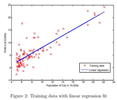
5. After you are finished, ex1.m will use your final parameters to plot the linear fit. The result should look something like Figure 2:




6. Your final values for θ will also be used to make predictions on profits in areas of 35,000 and 70,000 people. Note the way that the following lines in ex1.m uses matrix multiplication, rather than explicit summation or looping, to calculate the predictions. This is an example of code vectorization in Octave/MATLAB.

• In this part, you will fit the linear regression parameters θ to our dataset using gradient descent.




• Update Equations




1. The objective of linear regression is to minimize the cost function




2. \( J = \frac{1}{2m} \sum_{i=1}^{m} (h_{\theta}(x^{(i)}) - y^{(i)} )^2 \)




3. where the hypothesis hθ(x) is given by the linear mode




4. \( h_{\theta}(x) = \theta_0 + \theta_1(x) \)




5. Recall that the parameters of your model are the θj values. These are the values you will adjust to minimize cost J(θ). One way to do this is to use the batch gradient descent algorithm. In batch gradient descent, each iteration performs the update




6. \begin{align*} \text{repeat until convergence: } \lbrace & \newline \theta_0 := & \theta_0 - \alpha \frac{1}{m} \sum\limits_{i=1}^{m}(h_\theta(x_{i}) - y_{i}) \newline \theta_1 := & \theta_1 - \alpha \frac{1}{m} \sum\limits_{i=1}^{m}\left((h_\theta(x_{i}) - y_{i}) x_{i}\right) \newline \rbrace& \end{align*}




7. With each step of gradient descent, your parameters θj come closer to the optimal values that will achieve the lowest cost J(θ). Implementation Note: We store each example as a row in the the X matrix in Octave/MATLAB. To take into account the intercept term (θ0), we add an additional first column to X and set it to all ones. This allows us to treat θ0 as simply another ‘feature’.

• Perform all of these steps within the provided for-loop from 1 to the number of iterations. Note that the code template provides you this for-loop - you only have to complete the body of the for-loop. The steps below go immediately below where the script template says "======= YOUR CODE HERE ======".




• 1 - The hypothesis is a vector, formed by multiplying the X matrix and the theta vector. X has size (m x n), and theta is (n x 1), so the product is (m x 1). That's good, because it's the same size as 'y'. Call this hypothesis vector 'h'.




• 2 - The "errors vector" is the difference between the 'h' vector and the 'y' vector.




• 3 - The change in theta (the "gradient") is the sum of the product of X and the "errors vector", scaled by alpha and 1/m. Since X is (m x n), and the error vector is (m x 1), and the result you want is the same size as theta (which is (n x 1), you need to transpose X before you can multiply it by the error vector.




• The vector multiplication automatically includes calculating the sum of the products.




• When you're scaling by alpha and 1/m, be sure you use enough sets of parenthesis to get the factors correct.




• 4 - Subtract this "change in theta" from the original value of theta. A line of code like this will do it: theta = theta - theta_change;

• Test Case 1:
      
  >>[theta J_hist] = gradientDescent([1 5; 1 2; 1 4; 1 5],[1 6 4 2]',[0 0]',0.01,1000);
  
  % then type in these variable names, to display the final results
  >>theta
  theta =
      5.2148
     -0.5733
  >>J_hist(1)
  ans  =  5.9794
  >>J_hist(1000)
  ans = 0.85426
      
      
  For debugging, here are the first few theta values computed in the gradientDescent() for-loop for this test case:
      
  % first iteration 
  theta = 
     0.032500
     0.107500
  % second iteration
  theta = 
     0.060375
     0.194887
  % third iteration
  theta = 
     0.084476
     0.265867
  % fourth iteration
  theta = 
     0.10550
     0.32346
  
      
  The values can be inspected by adding the "keyboard" command within your for-loop. This exits the code to the debugger, where you can inspect the values. Use the "return" command to resume execution.
  
  Test Case 2:
  
  This test case is similar, but uses a non-zero initial theta value 
      
      
  >> [theta J_hist] = gradientDescent([1 5; 1 2],[1 6]',[.5 .5]',0.1,10);
  >> theta
  theta =
     1.70986
     0.19229
  
  >> J_hist
  J_hist =
     5.8853
     5.7139
     5.5475
     5.3861
     5.2294
     5.0773
     4.9295
     4.7861
     4.6469
     4.5117
     
      
  

1. Here are some things to keep in mind as you implement gradient descent: Octave/MATLAB array indices start from one, not zero. If you’re storing θ0 and θ1 in a vector called theta, the values will be theta(1) and theta(2).




2. If you are seeing many errors at runtime, inspect your matrix operations to make sure that you’re adding and multiplying matrices of compatible dimensions. Printing the dimensions of variables with the size command will help you debug.




3. 




4. By default, Octave/MATLAB interprets math operators to be matrix operators. This is a common source of size incompatibility errors. If you don’t want matrix multiplication, you need to add the “dot” notation to specify this to Octave/MATLAB. For example, A*B does a matrix multiply, while A.*B does an element-wise multiplication.




• Visualizing J(θ)




1. To understand the cost function J(θ) better, you will now plot the cost over a 2-dimensional grid of θ0 and θ1 values. You will not need to code anything new for this part, but you should understand how the code you have written already is creating these images.




2. In the next step of ex1.m, there is code set up to calculate J(θ) over a grid of values using the computeCost function that you wrote.




3. 
   % initialize J vals to a matrix of 0's
   J vals = zeros(length(theta0 vals), length(theta1 vals));
   % Fill out J vals
   for i = 1:length(theta0 vals)
   for j = 1:length(theta1 vals)
   t = [theta0 vals(i); theta1 vals(j)];
   J vals(i,j) = computeCost(x, y, t);
   end
   end
   




4. After these lines are executed, you will have a 2-D array of J(θ) values. The script ex1.m will then use these values to produce surface and contour plots of J(θ) using the surf and contour commands. The plots should look something like Figure 3:




5. 




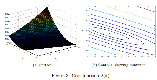
6. The purpose of these graphs is to show you that how J(θ) varies with changes in θ0 and θ1. The cost function J(θ) is bowl-shaped and has a global mininum. (This is easier to see in the contour plot than in the 3D surface plot). This minimum is the optimal point for θ0 and θ1, and each step of gradient descent moves closer to this point.