Introductory Video

The Machine Learning course includes several programming assignments which you’ll need to finish to complete the course. The assignments require the Octave scientific computing language.

Octave is a free, open-source application available for many platforms. It has a text interface and an experimental graphical one. Octave is distributed under the GNU Public License, which means that it is always free to download and distribute.

Use Download to install Octave for windows. "Warning: Do not install Octave 4.0.0";

Installing Octave on GNU/Linux : On Ubuntu, you can use: sudo apt-get update && sudo apt-get install octave. On Fedora, you can use: sudo yum install octave-forge

Files included in this exercise can be downloaded here ⇒ : Download

ex2.m - Octave/MATLAB script that steps you through the exercise

ex2_reg.m - Octave/MATLAB script for the later parts of the exercise

ex2data1.txt - Training set for the first half of the exercise

ex2data2.txt - Training set for the second half of the exercise

mapFeature.m- Function to generate polynomial features

plotDecisionBoundary.m - Function to plot classifier’s decision boundary

Files you will need to modify as part of this assignment :

plotData.m - Function to plot 2D classification data

sigmoid.m - Sigmoid Function

costFunction.m - Logistic Regression Cost Function

predict.m - Logistic Regression Prediction Function

costFunctionReg.m - Regularized Logistic Regression Cost

In this part of the exercise, you will build a logistic regression model to predict whether a student gets admitted into a university.

Suppose that you are the administrator of a university department and you want to determine each applicant’s chance of admission based on their results on two exams.

You have historical data from previous applicants that you can use as a training set for logistic regression.

For each training example, you have the applicant’s scores on two exams and the admissions decision.

Your task is to build a classification model that estimates an applicant’s probability of admission based the scores from those two exams.

This outline and the framework code in ex2.m will guide you through the exercise.

In the first part of ex2.m, the code will load the data and display it on a 2-dimensional plot by calling the function plotData.

You will now complete the code in plotData so that it displays a figure like Figure 1, where the axes are the two exam scores, and the positive and negative examples are shown with different markers

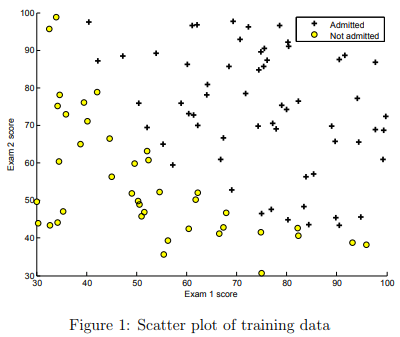
To help you get more familiar with plotting, we have left plotData.m empty so you can try to implement it yourself. However, this is an optional (ungraded) exercise. We also provide our implementation below so you can copy it or refer to it. If you choose to copy our example, make sure you learn what each of its commands is doing by consulting the Octave/MATLAB documentation.

% Find Indices of Positive and Negative Examples
pos = find(y==1); neg = find(y == 0);
% Plot Examples
plot(X(pos, 1), X(pos, 2), 'k+','LineWidth', 2, 'MarkerSize', 7);
plot(X(neg, 1), X(neg, 2), 'ko', 'MarkerFaceColor', 'y', 'MarkerSize', 7);

Recall that the logistic regression hypothesis is defined as: \( h_{\theta}(x) = g(\theta^Tx) \)

where function g is the sigmoid function. The sigmoid function is defined as: \( g(z) = \frac{1}{1 + e^{-x}} \)

Tutorial for sigmoid()

You can get a one-line function for sigmoid(z) if you use only element-wise operators.

The exp() function is element-wise.

The addition operator is element-wise.

Use the element-wise division operator ./

Combine these elements with a few parenthesis, and operate only on the parameter 'z'. The return value 'g' will then be the same size as 'z', regardless of what data 'z' contains.

Test Cases for sigmoid()

>> sigmoid(-5)
ans =  0.0066929

>> sigmoid(0)
ans =  0.50000

>> sigmoid(5)
ans =  0.99331

>> sigmoid([4 5 6])
ans =

   0.98201   0.99331   0.99753

>> sigmoid([-1;0;1])
ans =

   0.26894
   0.50000
   0.73106

>> V = reshape(-1:.1:.9, 4, 5);
>> sigmoid(V)
ans =

   0.26894   0.35434   0.45017   0.54983   0.64566
   0.28905   0.37754   0.47502   0.57444   0.66819
   0.31003   0.40131   0.50000   0.59869   0.68997
   0.33181   0.42556   0.52498   0.62246   0.71095

Now you will implement the cost function and gradient for logistic regression. Complete the code in costFunction.m to return the cost and gradient.

Recall that the cost function in logistic regression is

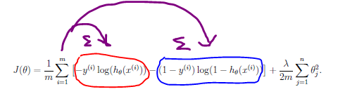
\( J(\theta) = − \frac{1}{m} \sum_{i = 1}^{m} [y^{(i)}log(h_{\theta}(x^{(i)}))−(1−y^{(i)})log(1−h_{\theta}(x^{(i)})) ] \)

and the gradient of the cost is a vector of the same length as θ where the j th element (for j = 0, 1, . . . , n) is defined as follows:

\( \theta := \theta − \frac{\alpha}{m} X^T (g(X\theta) - \overline{y} ) \)

Note that while this gradient looks identical to the linear regression gradient, the formula is actually different because linear and logistic regression have different definitions of hθ(x).

Once you are done, ex2.m will call your costFunction using the initial parameters of θ. You should see that the cost is about 0.693.

Tutorial: vectorizing the Cost function :

The hypothesis is a vector, formed from the sigmoid() of the products of X and \thetaθ. See the equation on ex2.pdf - Page 4. Be sure your sigmoid() function passes the submit grader before going any further.

First focus on the circled portions of the cost equation. Each of these is a vector of size (m x 1). In the steps below we'll distribute the summation operation, as shown in purple, so we end up with two scalars (for the 'red' and 'blue' calculations).

The red-circled term is the sum of -y multiplied by the natural log of h. Note that the natural log function is log(). Don't use log10(). Since we want the sum of the products, we can use a vector multiplication.

The size of each argument is (m x 1), and we want the vector product to be a scalar, so use a transposition so that (1 x m) times (m x 1) gives a result of (1 x 1), a scalar.

The blue-circled term uses the same method, except that the two vectors are (1 - y) and the natural log of (1 - h).

Subtract the right-side term from the left-side term Scale the result by 1/m. This is the unregularized cost.

Test cases for costFunction() :

X = [ones(3,1) magic(3)];
y = [1 0 1]';
theta = [-2 -1 1 2]';

% un-regularized
[j g] = costFunction(theta, X, y)

% results
j = 4.6832

g =
  0.31722
  0.87232
  1.64812
  2.23787

The gradient calculation can be easily vectorized.

\( \theta := \theta − \frac{\alpha}{m} X^T (g(X\theta) - \overline{y} ) \)

Note that if we set \( \theta_0 \) to zero (in Step 3 below), the second equation is exactly equal to the first equation. So we can ignore the "j = 0" condition entirely, and just use the second equation.

Recall that the hypothesis vector h is the sigmoid() of the product of X and θ (see ex2.pdf - Page 4). You probably already calculated h for the cost J calculation.

The left-side term is the vector product of X and (h - y), scaled by 1/m. You'll need to transpose and swap the product terms so the result is (m x n)' times (m x 1) giving you a (n x 1) result. This is the unregularized gradient. Note that the vector product also includes the required summation.

Then set theta(1) to 0 (if you haven't already).

The grad value is the sum of the Step 2 and Step 4 results.

In the previous assignment, you found the optimal parameters of a linear regression model by implementing gradent descent.

You wrote a cost function and calculated its gradient, then took a gradient descent step accordingly.

This time, instead of taking gradient descent steps, you will use an Octave/- MATLAB built-in function called fminunc.

Octave/MATLAB’s fminunc is an optimization solver that finds the minimum of an unconstrained function.

Constraints in optimization often refer to constraints on the parameters, for example, constraints that bound the possible values θ can take (e.g., θ ≤ 1).

Logistic regression does not have such constraints since θ is allowed to take any real value.

For logistic regression, you want to optimize the cost function J(θ) with parameters θ.

Concretely, you are going to use fminunc to find the best parameters θ for the logistic regression cost function, given a fixed dataset (of X and y values). You will pass to fminunc the following inputs:

The initial values of the parameters we are trying to optimize. A function that, when given the training set and a particular θ, computes the logistic regression cost and gradient with respect to θ for the dataset (X, y)

In ex2.m, we already have code written to call fminunc with the correct

% Set options for fminunc
options = optimset('GradObj', 'on', 'MaxIter', 400);
% Run fminunc to obtain the optimal theta
% This function will return theta and the cost
[theta, cost] = fminunc(@(t)(costFunction(t, X, y)), initial theta, options);

In this code snippet, we first defined the options to be used with fminunc. Specifically, we set the GradObj option to on, which tells fminunc that our function returns both the cost and the gradient. This allows fminunc to use the gradient when minimizing the function. Furthermore, we set the MaxIter option to 400, so that fminunc will run for at most 400 steps before it terminates.

To specify the actual function we are minimizing, we use a “short-hand” for specifying functions with the @(t) ( costFunction(t, X, y) ) . This creates a function, with argument t, which calls your costFunction. This allows us to wrap the costFunction for use with fminunc.

If you have completed the costFunction correctly, fminunc will converge on the right optimization parameters and return the final values of the cost and θ. Notice that by using fminunc, you did not have to write any loops yourself, or set a learning rate like you did for gradient descent.

This is all done by fminunc: you only needed to provide a function calculating the cost and the gradient.

Once fminunc completes, ex2.m will call your costFunction function using the optimal parameters of θ. You should see that the cost is about 0.203.

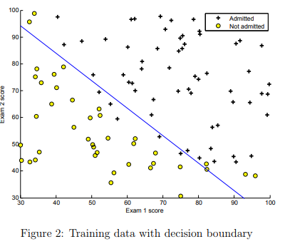
This final θ value will then be used to plot the decision boundary on the training data, resulting in a figure similar to Figure 2. We also encourage you to look at the code in plotDecisionBoundary.m to see how to plot such a boundary using the θ values

After learning the parameters, you can use the model to predict whether a particular student will be admitted.

For a student with an Exam 1 score of 45 and an Exam 2 score of 85, you should expect to see an admission probability of 0.776.

Another way to evaluate the quality of the parameters we have found is to see how well the learned model predicts on our training set. In this

part, your task is to complete the code in predict.m. The predict function will produce “1” or “0” predictions given a dataset and a learned parameter vector θ.

After you have completed the code in predict.m, the ex2.m script will proceed to report the training accuracy of your classifier by computing the percentage of examples it got correct.

Tutorial for ex2: predict()

This is logistic regression, so the hypothesis is the sigmoid of the product of X and theta.

Logistic prediction when there are only two classes uses a threshold of >= 0.5 to represent 1's and < 0.5 to represent a 0.

Here's an example of how to make this conversion in a vectorized manner. Try these commands in your workspace console, and study how they work:

v = rand(10,1)      % creates some random values between 0 and 1
v >= 0.5            % performs a logical comparison on each value

Inside your predict.m script, you will need to assign the results of this sort of logical comparison to the 'p' variable. You can use "p = " followed by a logical comparison inside a set of parenthesis.

Test Cases for predict()

>> X = [1 1 ; 1 2.5 ; 1 3 ; 1 4];
>> theta = [-3.5 ; 1.3];

% test case for predict()
>> predict(theta, X)
ans =

   0
   0
   1
   1

Setting Up Your Programming Assignment Environment

Introductory Video

Programming Exercise 3: Logistic Regression

Programming Exercise 3: Logistic Regression

Programming Exercise 3 Step 1 : Visualizing the data

Programming Exercise 3 Step 2 : sigmoid function

Programming Exercise 3 Step 3 : Cost function and gradient

Programming Exercise 3 Step 4 : Gradient

Programming Exercise 3 Step 5 : Learning parameters using fminunc

Programming Exercise 3 Step 6 : Evaluating logistic regression